Course3-Week2-推荐系统-程序员宅基地
技术标签: 深度学习 # 机器学习-吴恩达-完结 人工智能 推荐算法
Course3-Week2-推荐系统
文章目录
- 笔记主要参考B站视频“(强推|双字)2022吴恩达机器学习Deeplearning.ai课程”。
- 该课程在Course上的页面:Machine Learning 专项课程
- 课程资料:“UP主提供资料(Github)”、或者“我的下载(百度网盘)”。
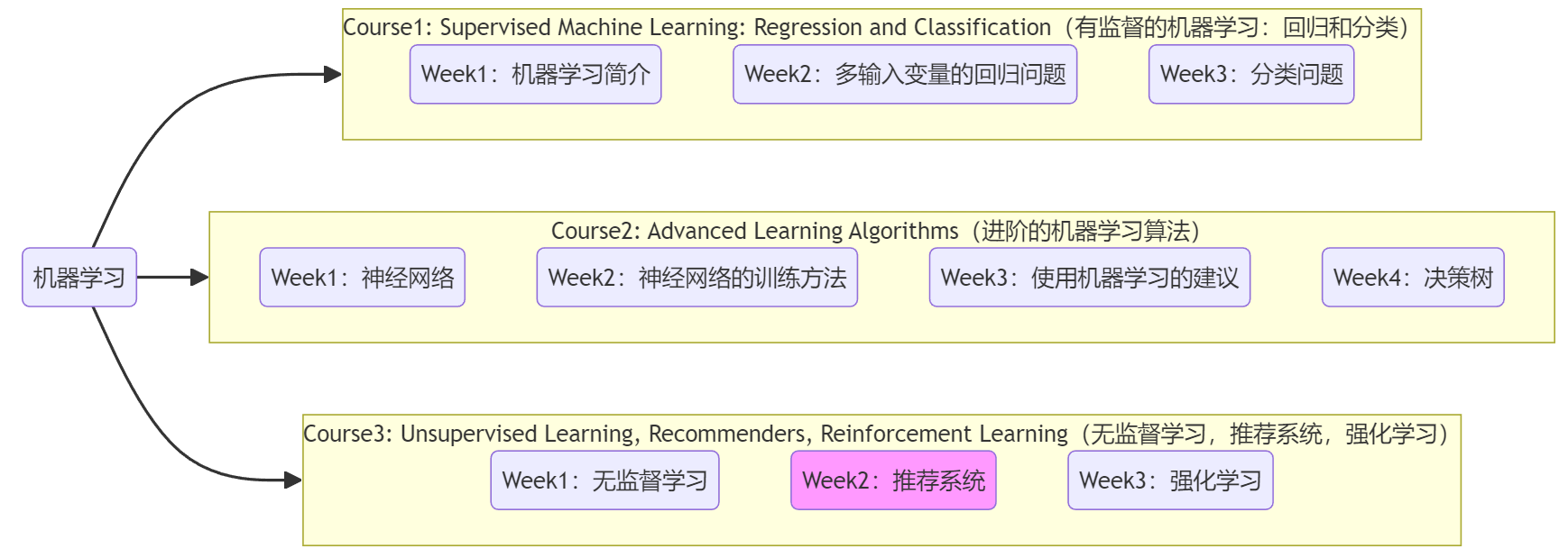
- 本篇笔记对应课程 Course3-Week2(下图中深紫色)。
1. 推荐机制的问题引入
本周将学习两种推荐算法“协同过滤算法”、“基于内容过滤”,由于都使用有标记的训练数据所以可以认为是“有监督学习”,但注意某些情况下这些算法的变体可能是“无监督学习”。尽管推荐算法在学术界相对没有那么热门,但是其商业应用十分广泛。比如,当访问在线购物网站(如淘宝)、流视频媒体平台(如B站、抖音)、音乐应用(如QQ音乐)时,通常都会有“为你推荐/猜你喜欢”的功能。对于很多公司来说,“推荐系统”和公司利润息息相关,所以很多大公司都会自行研发“推荐系统”。下面就来介绍其工作原理。
1.1 预测电影评分
本小节介绍一个贯穿本周的“推荐系统”案例——“预测电影评分”。
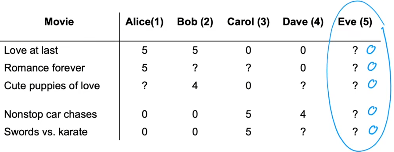
【问题1】“预测电影评分”:给出下面的数据集,预测用户对于没有看过的电影的评分。进而可以“为你推荐”。
注1:若无特殊说明,默认用户对电影的评分为(0,1,2,3,4,5)这6种分数。
注2:问号“?”表示用户并没有看过当前电影,也就没有评分。
注3:一般的推荐问题中,会将研究对象称为“item”,比如本例中就是“电影”。

1.2 数学符号
下面是本周会用到的一些数学符号,简单看一眼,用到的时候来查就行。
- n u n_u nu:用户的数量,并使用 j j j 表示单个用户索引。
- n m n_m nm:电影的数量,并使用 i i i 表示单个电影索引。
- n n n:电影的特征数量。
- w ⃗ ( j ) \vec{w}^{(j)} w(j)、 b ( j ) b^{(j)} b(j):第 j j j 个用户的参数,前者为 1 × n 1\times n 1×n 一维向量,后者为一个数。
- W W W、 b ⃗ \vec{b} b:所有的用户参数,前者为 n u × n n_u\times n nu×n 二维矩阵,后者为 1 × n 1\times n 1×n 一维向量。
- X X X: n m × n n_m\times n nm×n 二维矩阵,所有的电影特征。
- x ⃗ ( i ) \vec{x}^{(i)} x(i): 1 × n 1\times n 1×n 一维向量,第 i i i 个电影的特征。
- r ( i , j ) r(i,j) r(i,j):二元取值,表示用户 j j j 已经对电影 i i i 进行打分(1)、或者是没打分(0)。
- y ( i , j ) y^{(i,j)} y(i,j):一个值,表示用户 j j j 对电影 i i i 的评分。
- m ( j ) m^{(j)} m(j):一个值,表示用户 j j j 已经评分的电影总数。
本节 Quiz:You have the following table of movie ratings:
Movie Elissa zach Barry Terry Football Forever 5 4 3 ? Pies, Pies, Pies 1 ? 5 4 Linear Algebra Live 4 5 ? 1
Refer to the table above. Assume numbering starts at 1 for this quiz, so the rating for “Football Forever” by Elissa is at (1,1). What is the value of n u n_u nu?
Answer: 4Refer to the table above. What is the value of r ( 2 , 2 ) r(2,2) r(2,2)?
Answer: 0
2. 协同过滤算法
2.1 协同过滤算法-线性回归
本小节按照“线性回归”的思路层层递进,介绍“协同过滤算法”的基本步骤。
1. 使用“电影特征”计算“用户参数”

- x 1 x_1 x1:假设表示电影的“浪漫”程度。
- x 2 x_2 x2:假设表示电影的“打斗激烈”程度。
- x ⃗ ( i ) = [ x 1 ( i ) , x 2 ( i ) ] \vec{x}^{(i)}=[x_1^{(i)},x_2^{(i)}] x(i)=[x1(i),x2(i)]:表示电影 i i i 的特征。
假设我们目前完全已知电影的特征。那显然就可以直接使用“线性回归”,假设用户 j j j 对电影 i i i 的评分为 y ^ ( i , j ) = w ⃗ ( j ) x ⃗ ( i ) + b ( j ) \hat{y}^{(i,j)} = \vec{w}^{(j)}\vec{x}^{(i)}+b^{(j)} y^(i,j)=w(j)x(i)+b(j),于是便可最小化代价函数求解用户 j j j 的参数 w ⃗ ( j ) \vec{w}^{(j)} w(j)、 b ( j ) b^{(j)} b(j)。下面给出模型及单个用户的代价函数、全体用户的代价函数:
Linear model : y ^ ( i , j ) = w ⃗ ( j ) x ⃗ ( i ) + b ( j ) Cost function of user j : min w ⃗ j , b ( j ) J ( w ⃗ j , b ( j ) ) = 1 2 m ( j ) ∑ i : r ( i , j ) ( w ⃗ ( j ) x ⃗ ( i ) + b ( j ) − y ( i , j ) ) 2 + λ 2 m ( j ) ∑ k = 1 n ( w k ( j ) ) 2 Cost function of ALL users: min W , b ⃗ J ( W , b ⃗ ) = 1 2 ∑ j = 1 n u ∑ i : r ( i , j ) = 1 ( w ⃗ ( j ) x ⃗ ( i ) + b ( j ) − y ( i , j ) ) 2 + λ 2 ∑ j = 1 n u ∑ k = 1 n ( w k ( j ) ) 2 \begin{aligned} \text{Linear model :}&\quad \hat{y}^{(i,j)} = \vec{w}^{(j)}\vec{x}^{(i)}+b^{(j)}\\ \text{Cost function of user j :}&\quad \min_{\vec{w}^{j},b^{(j)}} J(\vec{w}^{j},b^{(j)}) = \frac{1}{2m^{(j)}}\sum_{i:\; r(i,j)}(\vec{w}^{(j)}\vec{x}^{(i)}+b^{(j)}-y^{(i,j)})^2 \textcolor{orange}{+\frac{\lambda}{2m^{(j)}}\sum_{k=1}^n(w_k^{(j)})^2}\\ \text{Cost function of ALL users:}&\quad \min_{W,\vec{b}} J(W,\vec{b}) = \frac{1}{2}\sum_{j=1}^{n_u}\sum_{i:\; r(i,j)=1}(\vec{w}^{(j)}\vec{x}^{(i)}+b^{(j)}-y^{(i,j)})^2 \textcolor{orange}{+\frac{\lambda}{2}\sum_{j=1}^{n_u}\sum_{k=1}^n(w_k^{(j)})^2} \end{aligned} Linear model :Cost function of user j :Cost function of ALL users:y^(i,j)=w(j)x(i)+b(j)wj,b(j)minJ(wj,b(j))=2m(j)1i:r(i,j)∑(w(j)x(i)+b(j)−y(i,j))2+2m(j)λk=1∑n(wk(j))2W,bminJ(W,b)=21j=1∑nui:r(i,j)=1∑(w(j)x(i)+b(j)−y(i,j))2+2λj=1∑nuk=1∑n(wk(j))2
注意正则化项没有参数 b b b,是因为加上也没影响。并且,代价函数分母上的 m ( j ) m^{(j)} m(j) 是个常数,对于最小化代价函数的过程没有影响,所以在全体用户的代价函数中直接省略掉。这一小节和之前的“线性回归”完全相同,只是在最后将代价函数推广到全体用户。
2. 使用“用户参数”计算“电影特征”

那现在假设我们不知道电影特征,但是完全已知用户参数。显然根据上一段给出的“线性回归”模型,我们也可以使用“用户参数”来计算“电影特征”。仿照上一段,模型和代价函数如下(代价函数误差项的不同仅在求和符号上):
Linear Model : y ^ ( i , j ) = w ⃗ ( j ) x ⃗ ( i ) + b ( j ) Cost function of movie i : min x ⃗ ( i ) J ( x ⃗ ( i ) ) = 1 2 ∑ j : r ( i , j ) ( w ⃗ ( j ) x ⃗ ( i ) + b ( j ) − y ( i , j ) ) 2 + λ 2 ∑ k = 1 n ( x k ( i ) ) 2 Cost function of ALL movies : min X J ( X ) = 1 2 ∑ i = 1 n m ∑ j : r ( i , j ) = 1 ( w ⃗ ( j ) x ⃗ ( i ) + b ( j ) − y ( i , j ) ) 2 + λ 2 ∑ j = 1 n m ∑ k = 1 n ( x k ( i ) ) 2 \begin{aligned} \text{Linear Model :}&\quad \hat{y}^{(i,j)} = \vec{w}^{(j)}\vec{x}^{(i)}+b^{(j)}\\ \text{Cost function of movie i :}&\quad \min_{\vec{x}^{(i)}} J(\vec{x}^{(i)}) = \frac{1}{2}\sum_{\textcolor{red}{j}:\; r(i,j)}(\vec{w}^{(j)}\vec{x}^{(i)}+b^{(j)}-y^{(i,j)})^2 \textcolor{orange}{+\frac{\lambda}{2}\sum_{k=1}^n(x_k^{(i)})^2}\\ \text{Cost function of ALL movies :}&\quad \min_{X} J(X) = \frac{1}{2}\sum_{\textcolor{red}{i=1}}^{\textcolor{red}{n_m}}\sum_{\textcolor{red}{j}:\; r(i,j)=1}(\vec{w}^{(j)}\vec{x}^{(i)}+b^{(j)}-y^{(i,j)})^2 \textcolor{orange}{+\frac{\lambda}{2}\sum_{j=1}^{n_m}\sum_{k=1}^n(x_k^{(i)})^2} \end{aligned} Linear Model :Cost function of movie i :Cost function of ALL movies :y^(i,j)=w(j)x(i)+b(j)x(i)minJ(x(i))=21j:r(i,j)∑(w(j)x(i)+b(j)−y(i,j))2+2λk=1∑n(xk(i))2XminJ(X)=21i=1∑nmj:r(i,j)=1∑(w(j)x(i)+b(j)−y(i,j))2+2λj=1∑nmk=1∑n(xk(i))2
在本周之前的线性回归中,“很多电影特征”只对应“一个用户”的信息,所以显然不能根据“用户参数”倒推“电影特征”(无穷解)。但现在有“很多用户”都对“同一个电影”做出了评分,于是就可以利用所有人的数据来计算电影特征。直观上来说,一个人的数据价值不大,但是很多人的数据可以倒推系统的某些参数,这体现了“大数据”的价值。
3. 协同过滤算法
实际情况中,我们不可能提前得知电影特征、用户参数的大小。现在我们假设电影特征 x ⃗ ( i ) \vec{x}^{(i)} x(i)、用户参数 w ⃗ ( j ) \vec{w}^{(j)} w(j)的长度为2,于是将上面两种情况综合起来,根据已知的的用户评分,来协同求解未知的电影特征、用户参数,就是“协同过滤算法(Collaborative filtering)”。注意到,“所有用户的代价函数”、“所有电影的代价函数”中的“平方误差项”完全相同,都使用到了所有用户已经打分的数据,于是便可以考虑将两者合并,再加上所有的正则项,即可得到完整的代价函数:
Linear Model : y ^ ( i , j ) = f W , b ⃗ , X ( x ⃗ ( i ) ) = w ⃗ ( j ) x ⃗ ( i ) + b ( j ) Cost function of ALL users and ALL movies: min W , b ⃗ , X J ( W , b ⃗ , X ) = 1 2 ∑ ( i , j ) : r ( i , j ) = 1 ( w ⃗ ( j ) x ⃗ ( i ) + b ( j ) − y ( i , j ) ) 2 + λ 2 ∑ j = 1 n u ∑ k = 1 n ( w k ( j ) ) 2 + λ 2 ∑ j = 1 n m ∑ k = 1 n ( x k ( i ) ) 2 Gradient descent repeat until convergence : { i = 1 , 2 , . . . , n m . j = 1 , 2 , . . . , n u . k = 1 , 2 , . . . , n . w k ( j ) = w k ( j ) − α ∂ ∂ w k ( j ) J ( W , b ⃗ , X ) b ( j ) = b ( j ) − α ∂ ∂ b ( j ) J ( W , b ⃗ , X ) x k ( i ) = x k ( i ) − α ∂ ∂ x k ( i ) J ( W , b ⃗ , X ) \begin{aligned} & \text{Linear Model :} \quad \hat{y}^{(i,j)} = f_{W,\vec{b},X}(\vec{x}^{(i)}) = \vec{w}^{(j)}\vec{x}^{(i)}+b^{(j)}\\ &\text{Cost function of ALL users and ALL movies:} \\ \quad &\min_{W,\vec{b}, X} J(W,\vec{b}, X) = \frac{1}{2}\sum_{(i,j):\; r(i,j)=1}(\vec{w}^{(j)}\vec{x}^{(i)}+b^{(j)}-y^{(i,j)})^2 \textcolor{orange}{+\frac{\lambda}{2}\sum_{j=1}^{n_u}\sum_{k=1}^n(w_k^{(j)})^2} \textcolor{orange}{+\frac{\lambda}{2}\sum_{j=1}^{n_m}\sum_{k=1}^n(x_k^{(i)})^2}\\ & \begin{aligned} \text{Gradient descent} \\ \text{repeat until convergence} \end{aligned} : \left\{\begin{aligned} i &= 1,2,...,n_m. \\ j &= 1,2,...,n_u. \\ k &= 1,2,...,n. \\ w^{(j)}_k &= w^{(j)}_k - \alpha \frac{\partial }{\partial w^{(j)}_k} J(W,\vec{b}, X) \\ b^{(j)} &= b^{(j)} - \alpha \frac{\partial }{\partial b^{(j)}} J(W,\vec{b}, X)\\ x^{(i)}_k &= x^{(i)}_k - \alpha \frac{\partial }{\partial x^{(i)}_k} J(W,\vec{b}, X) \\ \end{aligned}\right. \end{aligned} Linear Model :y^(i,j)=fW,b,X(x(i))=w(j)x(i)+b(j)Cost function of ALL users and ALL movies:W,b,XminJ(W,b,X)=21(i,j):r(i,j)=1∑(w(j)x(i)+b(j)−y(i,j))2+2λj=1∑nuk=1∑n(wk(j))2+2λj=1∑nmk=1∑n(xk(i))2Gradient descentrepeat until convergence:⎩ ⎨ ⎧ijkwk(j)b(j)xk(i)=1,2,...,nm.=1,2,...,nu.=1,2,...,n.=wk(j)−α∂wk(j)∂J(W,b,X)=b(j)−α∂b(j)∂J(W,b,X)=xk(i)−α∂xk(i)∂J(W,b,X)
上述对代价函数应用“梯度下降法”求解偏导更新参数,不断逼近代价极小点即可得到最优参数。注意梯度下降法不只针对用户参数求偏导,而是需要同时使用偏导更新 w ⃗ ( j ) \vec{w}^{(j)} w(j)、 b ( j ) b^{(j)} b(j)、 x ⃗ ( i ) \vec{x}^{(i)} x(i) 所有参数。总结一下,“协同过滤算法”的整个过程就是,使用所有用户已经评分的数据,求解出所有的用户参数、所有的电影特征。
2.2 协同过滤算法-逻辑回归
事实上,很多“推荐算法”或者说是“协同过滤算法”都只使用“二进制标签”,来表示用户喜欢(1)、不喜欢(0),而不是可以给出连续取值的电影评分。比如下面给出了“二进制标签”的可能含义,包括但不限于短视频平台、社交软件、购物平台、广告推送等:
- 用户是否观看30s以上。或者说是完播率。
- 用户是否点赞或收藏。
- 用户是否购买了某种商品。
- 用户是否点击。
于是对于这种情况,就需要将“线性回归模型”转换成“逻辑回归模型”,代价函数中的“平方误差”也要转换成“二元交叉熵”:
Logistic model : y ^ ( i , j ) = f W , b ⃗ , X ( x ⃗ ( i ) ) = g ( w ⃗ ( j ) x ⃗ ( i ) + b ( j ) ) = 1 1 + e − ( w ⃗ ( j ) x ⃗ ( i ) + b ( j ) ) Cost function : min W , b ⃗ , X J ( W , b ⃗ , X ) = ∑ ( i , j ) : r ( i , j ) = 1 m [ − y ( i , j ) log ( y ^ ( i , j ) ) − ( 1 − y ( i , j ) ) log ( 1 − y ^ ( i , j ) ) ] + λ 2 ∑ j = 1 n u ∑ k = 1 n ( w k ( j ) ) 2 + λ 2 ∑ j = 1 n m ∑ k = 1 n ( x k ( i ) ) 2 , Gradient descent repeat until convergence : { i = 1 , 2 , . . . , n m . j = 1 , 2 , . . . , n u . k = 1 , 2 , . . . , n . w k ( j ) = w k ( j ) − α ∂ ∂ w k ( j ) J ( W , b ⃗ , X ) b ( j ) = b ( j ) − α ∂ ∂ b ( j ) J ( W , b ⃗ , X ) x k ( i ) = x k ( i ) − α ∂ ∂ x k ( i ) J ( W , b ⃗ , X ) \begin{aligned} &\text{Logistic model :} \quad \hat{y}^{(i,j)} = f_{W,\vec{b},X}(\vec{x}^{(i)}) = g(\vec{w}^{(j)}\vec{x}^{(i)}+b^{(j)})=\frac{1}{1+e^{-(\vec{w}^{(j)}\vec{x}^{(i)}+b^{(j)})}}\\ &\text{Cost function :} \min_{W,\vec{b},X} J(W,\vec{b},X) = \sum_{(i,j):\;r(i,j)=1}^{m}[-y^{(i,j)}\log(\hat{y}^{(i,j)})-(1-y^{(i,j)})\log(1-\hat{y}^{(i,j)})] \\ &\qquad\qquad\qquad\qquad\qquad\qquad\qquad\qquad \textcolor{orange}{+\frac{\lambda}{2}\sum_{j=1}^{n_u}\sum_{k=1}^n(w_k^{(j)})^2} \textcolor{orange}{+\frac{\lambda}{2}\sum_{j=1}^{n_m}\sum_{k=1}^n(x_k^{(i)})^2},\\ &\begin{aligned} \begin{aligned} \text{Gradient descent} \\ \text{repeat until convergence} \end{aligned} : \left\{\begin{aligned} i &= 1,2,...,n_m. \\ j &= 1,2,...,n_u. \\ k &= 1,2,...,n. \\ w^{(j)}_k &= w^{(j)}_k - \alpha \frac{\partial }{\partial w^{(j)}_k} J(W,\vec{b}, X) \\ b^{(j)} &= b^{(j)} - \alpha \frac{\partial }{\partial b^{(j)}} J(W,\vec{b}, X)\\ x^{(i)}_k &= x^{(i)}_k - \alpha \frac{\partial }{\partial x^{(i)}_k} J(W,\vec{b}, X) \\ \end{aligned}\right. \end{aligned} \end{aligned} Logistic model :y^(i,j)=fW,b,X(x(i))=g(w(j)x(i)+b(j))=1+e−(w(j)x(i)+b(j))1Cost function :W,b,XminJ(W,b,X)=(i,j):r(i,j)=1∑m[−y(i,j)log(y^(i,j))−(1−y(i,j))log(1−y^(i,j))]+2λj=1∑nuk=1∑n(wk(j))2+2λj=1∑nmk=1∑n(xk(i))2,Gradient descentrepeat until convergence:⎩
⎨
⎧ijkwk(j)b(j)xk(i)=1,2,...,nm.=1,2,...,nu.=1,2,...,n.=wk(j)−α∂wk(j)∂J(W,b,X)=b(j)−α∂b(j)∂J(W,b,X)=xk(i)−α∂xk(i)∂J(W,b,X)
2.3 均值归一化
上面已经介绍“协同过滤算法”的线性回归形式和逻辑回归形式,但在执行这个算法之前,首先还需要进行数据预处理——“均值归一化(mean normalization)”,会使算法的效果更好。这是因为新用户没有对任何电影做出评分,于是对于“代价函数”中的“误差项”不起作用,再加上“正则项”会进行减小用户参数的影响,于是新用户的参数 w ⃗ ( j ) \vec{w}^{(j)} w(j)全为0(一般初始化 b ( j ) b^{(j)} b(j)为0),此时对于任何电影的评分也就是全是0。也就是说:
- 不进行“均值归一化”,新用户的默认评分全是0(全都不喜欢),这就没法推荐了。
- “均值归一化”后,新用户的默认评分是当前电影的平均评分。起码也可以默认推荐平均分较高的电影。
总结:“均值归一化”使得推荐算法对于新用户、很少评价电影的用户的预测更加准确。

下面是“均值归一化”的具体步骤:
- 对于每一个电影,计算出所给出已有评分的平均分: μ i = mean j : r ( i , j ) = 1 ( y ( i , j ) ) \mu_i = \underset{j:\;r(i,j)=1}{\text{mean}}(y^{(i,j)}) μi=j:r(i,j)=1mean(y(i,j))
- 将所有评分进行“均值归一化”: y ( i , j ) = y ( i , j ) − μ i y^{(i,j)} = y^{(i,j)}-\mu_i y(i,j)=y(i,j)−μi
- 正常进行“协同过滤算法”,预测出新的评分: f W , b ⃗ , X ( x ( i ) ) f_{W,\vec{b},X}(x^{(i)}) fW,b,X(x(i))
- 将均值加回,即为最后结果: y ^ ( i , j ) = f W , b ⃗ , X ( x ( i ) ) + μ j \hat{y}^{(i,j)} = f_{W,\vec{b},X}(x^{(i)}) + \mu_j y^(i,j)=fW,b,X(x(i))+μj
事实上,进行“均值归一化”后,“推荐算法”也会运行的更快一点,并且预测结果也更加合理。
那既然可以对“行”进行“均值归一化”,那对“列”有必要进行均值归一化吗?完全没必要!因为对于一个新电影来说,不必将其推给所有人观看,所以其特征可以全部默认为0,直到有人进行评分后再更新特征值即可。“均值归一化”的总结:
- 对行进行“均值归一化”【推荐】:使新用户的默认评分等于当前电影的平均分。
- 对列进行“均值归一化”【没必要】:使新电影的默认评分等于某个用户的平均分。
2.4 协同过滤算法的TensorFlow实现
本节介绍使用TensorFlow实现“协同过滤算法”的大致框架。由于“协同过滤算法”并没有封装好的函数,所以代价函数的计算过程需要我们手动定义,但是求解偏导则可以交给TensotFlow内置的“自动微分”机制完成。具体来说,主要使用 tensorflow.GradientTape()来定义代价函数的计算过程,并使用其 .gradient()方法计算偏导来完成迭代更新。下面给出两个代码示例:
注:“Auto-diff”也称为“Auto-Grad”,其他机器学习包也支持,如“PyTorch”。
#####################【示例1】#####################
# 使用梯度下降法迭代更新参数
# 代价函数:J=(wx-y)**2
##################################################
# 定义初始参数
w = tf.Variable(3.0) # 待优化参数,并给出初始值
x = 1.0              # 特征值
y = 1.0              # 目标值
alpha = 0.01         # 学习率
iterations = 30      # 迭代次数
# 迭代寻找代价函数最小值
for iter in range (iterations) :
    # 定义计算代价函数的步骤,方便后续的自动微分(auto-diff)。
    with tf.GradientTape() as tape:
        fwb = w*x
        costJ = (fwb - y)**2
    # 自动微分计算参数的偏导
    [dJdw] = tape.gradient(costJ, [w])
    # 对参数进行迭代更新
    w.assign_add(-alpha * dJdw)

#####################【示例2】#####################
# 使用Adam算法迭代更新参数
# 代价函数:自定义函数 myCostCal(),参考2.1节
# 给出参数:
#   X:二维矩阵,电影特征,每一行表示一个电影
#   W:二维矩阵,用户参数,每一行表示一个用户
#   b:一维向量,用户参数,每一个表示一个用户
#   Ynorm:二维矩阵,“均值归一化”后的打分
#   R:二维矩阵,表示哪些打分是有效的
#   lambda:正则化参数
##################################################
optimizer = keras.optimizers.Adam(learning_rate=1e-1)
iterations = 200
for iter in range (iterations) :
    # 定义如何计算代价函数
    with tf.GradientTape() as tape:
        # 自定义函数:使用前向传播写出代价函数的计算步骤
        cost_value = myCostCal(X, W, b,Ynorm, R, num_users, num_movies, lambda)
    # 计算代价函数对于所有待求参数的偏导
    grads = tape.gradient( cost_value, [X,W,b] )
    # 使用Adam函数中的方法更新参数
    optimizer.apply_gradients( zip(grads, [X,w,b]) )
2.5 寻找相似的电影、协同过滤算法的缺点
实际当我们浏览电影网站时,可能会有很多“相似产品”推荐,那如何评判两个电影(item)很相似呢?使用特征之间的距离平方进行衡量。比如判断 电影 p p p 和 电影 i i i 的相似程度就可以使用:
∥ x ⃗ ( p ) − x ⃗ ( i ) ∥ 2 = ∑ k = 1 n ( x k ( p ) − x k ( i ) ) 2 \lVert \vec{x}^{(p)}-\vec{x}^{(i)} \rVert^2 = \sum_{k=1}^{n}(x_k^{(p)}-x_k^{(i)})^2 ∥x(p)−x(i)∥2=k=1∑n(xk(p)−xk(i))2
这同时将有助于我们提前筛选大量的数据(见3.2节)。并且,如果我们直接推荐和用户评价的高分电影“相似”的电影,就成了“无监督学习”。
最后是 “协同过滤算法”的缺点:
- 不擅长解决“冷启动(cold start)”问题。当有一个新电影或者新用户时,“协同过滤算法”的预测值就不是很准确。虽然再2.3节的均值归一化给出了一定的解决思路,但是还有更好的方法。
- 无法使用“用户”或“项目”的附加信息。前面已经强调,我们并不能提前知道“用户参数”和“电影特征”的数量和含义,所以上述“协同过滤算法”类似于“盲算”。但实际上,我们可以知道电影的一些信息,比如类型、演员、出品方、预算等;也可以知道一些用户的信息,比如性别、年龄、地址、类型偏好、浏览器等。如何将这些“附加信息”利用到模型中也是需要考虑的问题。
下节介绍的“基于内容过滤”将解决上述问题。
2.6 代码示例-预测电影分数
本小节使用真实的电影评分数据集,来训练“协同过滤算法”。最后根据自己对某些电影的评分,预测自己感兴趣的电影。问题要求和代码结构如下:
问题要求:完成对数据集的“协同过滤算法”训练,并使用其预测自己的偏好。
代码结构:
- 函数:若干,后续再补充注释。
- 主函数:加载原始数据集,训练协同过滤算法,最后进行新用户预测。
注:本实验来自本周的练习“C3_W2_Collaborative_RecSys_Assignment.ipynb”。
注2:数据集见UP主提供的“课程资料”或者直接从百度网盘下载“C3-W2-2-6data(467KB)”。The data set is derived from the MovieLens “ml-latest-small” dataset.
[F. Maxwell Harper and Joseph A. Konstan. 2015. The MovieLens Datasets: History and Context. ACM Transactions on Interactive Intelligent Systems (TiiS) 5, 4: 19:1–19:19. https://doi.org/10.1145/2827872]
下面是代码和运行结果:
import numpy as np
from numpy import loadtxt

import tensorflow as tf
from tensorflow import keras

import pandas as pd
#############################################################################
def normalizeRatings(Y, R):
    """
    对电影评分进行均值归一化。注意只使用 R(i,j)=1 的评分计算均值。
    Args:
        Y:二维矩阵,记录所有的原始评分。每一行表示一个电影、每一列表示一个用户。
        R:二维矩阵,表示当前位置的评分是否有效。
    returns:
        Ynorm:二维矩阵,均值归一化后的评分。
        Ymean:一维向量,记录每个电影的平均评分。
    """
    Ymean = (np.sum(Y*R,axis=1)/(np.sum(R, axis=1)+1e-12)).reshape(-1,1)
    Ynorm = Y - np.multiply(Ymean, R)
    return(Ynorm, Ymean)

def load_precalc_params_small():
    """
    加载初始化的用户参数和电影特征:W、b、X
    """
    floder_path = 'C:/Users/14751/Desktop/机器学习-吴恩达/学习笔记'
    # 加载W
    file = open(floder_path+'/data/small_movies_W.csv', 'rb')
    W = loadtxt(file,delimiter = ",")
    # 加载b
    file = open(floder_path+'/data/small_movies_b.csv', 'rb')
    b = loadtxt(file,delimiter = ",")
    b = b.reshape(1,-1)
    # 加载X
    file = open(floder_path+'/data/small_movies_X.csv', 'rb')
    X = loadtxt(file, delimiter = ",")
    return(X, W, b)

def load_ratings_small():
    """
    加载评分相关的参数:Y、R
    """
    floder_path = 'C:/Users/14751/Desktop/机器学习-吴恩达/学习笔记'
    # 加载Y
    file = open(floder_path+'/data/small_movies_Y.csv', 'rb')
    Y = loadtxt(file,delimiter = ",")
    # 加载R
    file = open(floder_path+'/data/small_movies_R.csv', 'rb')
    R = loadtxt(file,delimiter = ",")
    return(Y,R)

def load_Movie_List_pd():
    """
    加载记录了“电影名称”、“平均评分”、“评分数量”等信息的表格。
    函数名中的“pd”表示使用了pands中的方法。
    returns df with and index of movies in the order they are in in the Y matrix
    """
    floder_path = 'C:/Users/14751/Desktop/机器学习-吴恩达/学习笔记'
    df = pd.read_csv(floder_path+'/data/small_movie_list.csv', header=0, index_col=0,  delimiter=',', quotechar='"')
    mlist = df["title"].to_list()
    return(mlist, df)

#############################################################################
def cofi_cost_func(X, W, b, Y, R, lambda_):
    """
    计算协同过滤算法的代价函数(有正则项)。
    Args:
      X (ndarray (num_movies,num_features)): matrix of item features
      W (ndarray (num_users,num_features)) : matrix of user parameters
      b (ndarray (1, num_users)            : vector of user parameters
      Y (ndarray (num_movies,num_users)    : matrix of user ratings of movies
      R (ndarray (num_movies,num_users)    : matrix, where R(i, j) = 1 if the i-th movies was rated by the j-th user
      lambda_ (float): regularization parameter
    Returns:
      J (float) : Cost
    """
    # # 方法一:使用numpy中的矩阵运算
    # yhat = np.matmul(X,W.T)+b
    # squ_error = (((yhat-Y)*R)**2).sum() / 2
    # regular_item = ((W**2).sum() + (X**2).sum()) / 2 * lambda_
    # return squ_error + regular_item

    # 方法二:使用TensorFlow中的矩阵运算
    yhat = tf.linalg.matmul(X, tf.transpose(W)) + b - Y
    J = 0.5 * tf.reduce_sum((yhat*R)**2) + (lambda_/2) * (tf.reduce_sum(X**2) + tf.reduce_sum(W**2))
    return J

###################################主函数##################################
# 加载原始数据集
# X, W, b = load_precalc_params_small()
# Y, R = load_ratings_small()
# num_movies, num_features = X.shape
# num_users,_ = W.shape
# print("Y", Y.shape, "R", R.shape)
# print("X", X.shape)
# print("W", W.shape)
# print("b", b.shape)
# print("num_features", num_features)
# print("num_movies",   num_movies)
# print("num_users",    num_users)

# 加载原始数据集
Y, R = load_ratings_small()
movieList, movieList_df = load_Movie_List_pd()

# 设置新用户的偏好
my_ratings = np.zeros(Y.shape[0])  #  Initialize my ratings
# Check the file small_movie_list.csv for id of each movie in our dataset
# We have selected a few movies we liked / did not like and the ratings we
# gave are as follows:
my_ratings[2700] = 5   # Toy Story 3 (2010)
my_ratings[2609] = 2   # Persuasion (2007)
my_ratings[929]  = 5   # Lord of the Rings: The Return of the King, The
my_ratings[246]  = 5   # Shrek (2001)
my_ratings[2716] = 3   # Inception
my_ratings[1150] = 5   # Incredibles, The (2004)
my_ratings[382]  = 2   # Amelie (Fabuleux destin d'Amélie Poulain, Le)
my_ratings[366]  = 5   # Harry Potter and the Sorcerer's Stone (a.k.a. Harry Potter and the Philosopher's Stone) (2001)
my_ratings[622]  = 5   # Harry Potter and the Chamber of Secrets (2002)
my_ratings[988]  = 3   # Eternal Sunshine of the Spotless Mind (2004)
my_ratings[2925] = 1   # Louis Theroux: Law & Disorder (2008)
my_ratings[2937] = 1   # Nothing to Declare (Rien à déclarer)
my_ratings[793]  = 5   # Pirates of the Caribbean: The Curse of the Black Pearl (2003)
my_rated = [i for i in range(len(my_ratings)) if my_ratings[i] > 0]
# 输出新用户的评分
print('新用户的评分有:')
for i in range(len(my_ratings)):
    if my_ratings[i] > 0 :
        print(f'Rated {
      my_ratings[i]} for  {
      movieList_df.loc[i,"title"]}');

# 将新用户评分新增到数据集中
Y    = np.c_[my_ratings, Y]
R    = np.c_[(my_ratings != 0).astype(int), R]
num_movies, num_users = Y.shape
num_features = 100

# 均值归一化
Ynorm, Ymean = normalizeRatings(Y, R)

# 使用tf.Variable初始化参数:W、X、b
tf.random.set_seed(1234) # for consistent results
W = tf.Variable(tf.random.normal((num_users,  num_features),dtype=tf.float64),  name='W')
X = tf.Variable(tf.random.normal((num_movies, num_features),dtype=tf.float64),  name='X')
b = tf.Variable(tf.random.normal((1,          num_users),   dtype=tf.float64),  name='b')

# 使用“协同过滤算法”迭代训练参数:W、X、b
optimizer = keras.optimizers.Adam(learning_rate=1e-1)
iterations = 200 # 迭代次数
lambda_ = 1      # 代价函数的正则化参数
print("\n开始进行训练:")
for iter in range(iterations):
    # 定义代价函数计算过程
    with tf.GradientTape() as tape:
        # 计算代价的大小
        cost_value = cofi_cost_func(X, W, b, Ynorm, R, lambda_)

    # 定义需要求解哪些参数的偏导
    grads = tape.gradient( cost_value, [X,W,b] )

    # Adam算法更新参数
    optimizer.apply_gradients( zip(grads, [X,W,b]) )

    # 展示迭代进度及代价
    if iter % 20 == 0:
        print(f"Training loss at iteration {
      iter}: {
      cost_value:0.1f}")


# 使用上述训练好的参数进行预测
p = np.matmul(X.numpy(), np.transpose(W.numpy())) + b.numpy()
pm = p + Ymean
my_predictions = pm[:,0]
# 预测评分和原始评分的对比
print('\n新用户的原始评分 vs 预测评分:')
for i in range(len(my_ratings)):
    if my_ratings[i] > 0:
        print(f'Original {
      my_ratings[i]}, Predicted {
      my_predictions[i]:0.2f} for {
      movieList[i]}')
# 预测用户最喜欢的电影
ix = tf.argsort(my_predictions, direction='DESCENDING')
print("\n下面是预测评分Top17中没看过的电影:")
for i in range(17):
    j = ix[i]
    if j not in my_rated:
        print(f'Predicting rating {
      my_predictions[j]:0.2f} for movie {
      movieList[j]}')
新用户的评分有:
Rated 5.0 for  Shrek (2001)
Rated 5.0 for  Harry Potter and the Sorcerer's Stone (a.k.a. Harry Potter and the Philosopher's Stone) (2001)
Rated 2.0 for  Amelie (Fabuleux destin d'Amélie Poulain, Le) (2001)
Rated 5.0 for  Harry Potter and the Chamber of Secrets (2002)
Rated 5.0 for  Pirates of the Caribbean: The Curse of the Black Pearl (2003)
Rated 5.0 for  Lord of the Rings: The Return of the King, The (2003)
Rated 3.0 for  Eternal Sunshine of the Spotless Mind (2004)
Rated 5.0 for  Incredibles, The (2004)
Rated 2.0 for  Persuasion (2007)
Rated 5.0 for  Toy Story 3 (2010)
Rated 3.0 for  Inception (2010)
Rated 1.0 for  Louis Theroux: Law & Disorder (2008)
Rated 1.0 for  Nothing to Declare (Rien à déclarer) (2010)
2023-12-14 16:58:16.542280: I tensorflow/core/platform/cpu_feature_guard.cc:182] This TensorFlow binary is optimized to use available CPU instructions in performance-critical operations.
To enable the following instructions: SSE SSE2 SSE3 SSE4.1 SSE4.2 AVX2 FMA, in other operations, rebuild TensorFlow with the appropriate compiler flags.

开始进行训练:
Training loss at iteration 0: 2321191.3
Training loss at iteration 20: 136169.3
Training loss at iteration 40: 51863.7
Training loss at iteration 60: 24599.0
Training loss at iteration 80: 13630.6
Training loss at iteration 100: 8487.7
Training loss at iteration 120: 5807.8
Training loss at iteration 140: 4311.6
Training loss at iteration 160: 3435.3
Training loss at iteration 180: 2902.1

新用户的原始评分 vs 预测评分:
Original 5.0, Predicted 4.90 for Shrek (2001)
Original 5.0, Predicted 4.84 for Harry Potter and the Sorcerer's Stone (a.k.a. Harry Potter and the Philosopher's Stone) (2001)
Original 2.0, Predicted 2.13 for Amelie (Fabuleux destin d'Amélie Poulain, Le) (2001)
Original 5.0, Predicted 4.88 for Harry Potter and the Chamber of Secrets (2002)
Original 5.0, Predicted 4.87 for Pirates of the Caribbean: The Curse of the Black Pearl (2003)
Original 5.0, Predicted 4.89 for Lord of the Rings: The Return of the King, The (2003)
Original 3.0, Predicted 3.00 for Eternal Sunshine of the Spotless Mind (2004)
Original 5.0, Predicted 4.90 for Incredibles, The (2004)
Original 2.0, Predicted 2.11 for Persuasion (2007)
Original 5.0, Predicted 4.80 for Toy Story 3 (2010)
Original 3.0, Predicted 3.00 for Inception (2010)
Original 1.0, Predicted 1.41 for Louis Theroux: Law & Disorder (2008)
Original 1.0, Predicted 1.26 for Nothing to Declare (Rien à déclarer) (2010)

下面是预测评分Top17中没看过的电影:
Predicting rating 4.49 for movie My Sassy Girl (Yeopgijeogin geunyeo) (2001)
Predicting rating 4.48 for movie Martin Lawrence Live: Runteldat (2002)
Predicting rating 4.48 for movie Memento (2000)
Predicting rating 4.47 for movie Delirium (2014)
Predicting rating 4.47 for movie Laggies (2014)
Predicting rating 4.47 for movie One I Love, The (2014)
Predicting rating 4.46 for movie Particle Fever (2013)
Predicting rating 4.45 for movie Eichmann (2007)
Predicting rating 4.45 for movie Battle Royale 2: Requiem (Batoru rowaiaru II: Chinkonka) (2003)
Predicting rating 4.45 for movie Into the Abyss (2011)
本节 Quiz:
- In which of the following situations will a collaborative filtering system be the most appropriate learning algorithm (compared to linear or logistic regression)?
× You subscribe to an online video streaming service, and are not satisfied with their movie suggestions. You download all your viewing for the last 10 years and rate each item. You assign each item a genre. Using your ratings and genre assignment, you learn to predict how you will rate new movies based on the genre.
错误点:只预测自己。
√ You run an online bookstore and collect the ratings of many users. You want to use this to identify what books are “similar” to each other (i.e, if a user likes a certain book, what are other books that they might also like?)
× You’re an artist and hand-paint portraits for your clients. Each client gets a different portrait (of themselves) and gives you 1-5 star rating feedback, and each client purchases at most 1 portrait. You’d like to predict what rating your next customer will give you.
错误点:每个人只给自己打分。
× You manage an online bookstore and you have the book ratings from many users. You want to learn to predict the expected sales volume (number of books sold) as a function of the average rating of a book.
错误点:预测的不是某个人的打分,而是整体销售量。注:“协同过滤”算法的核心思想在于用户参数、电影特征之间相互计算,所以很多用户都对很多作品打分。
For recommender systems with binary labels y y y, which of these are reasonable ways for defining when y y y should be 1 for a given user j j j and item i i i? (Check all that apply.)
√ y y y is 1 if user j j j purchases item i i i (after being shown the item).
√ y y y is 1 if user j j j fav/likes/clicks on item i i i (after being shown the item).
× y y y is 1 if user j j j has been shown item i i i by the recommendation engine.
× y y y is 1 if user j j j has not yet been shown item i i i by the recommendation engine.Lecture described using ‘mean normalization’ to do feature scaling of the ratings. What equation below best describes this algorithm?
× y n o r m ( i , j ) = y ( i , j ) − μ i m a x i − m i n i where μ i = ∑ j : r ( i , j ) = 1 y ( i , j ) ∑ j r ( i , j ) y_{norm}(i,j)=\frac{y(i,j)-\mu_i}{max_i-min_i}\;\;\text{where}\;\;\mu_i=\frac{\sum_{j:r(i,j)=1}y(i,j)}{\sum_j r(i,j)} ynorm(i,j)=maxi−miniy(i,j)−μiwhereμi=∑jr(i,j)∑j:r(i,j)=1y(i,j)
× y n o r m ( i , j ) = y ( i , j ) − μ i σ i where μ i = ∑ j : r ( i , j ) = 1 y ( i , j ) ∑ j r ( i , j ) , σ i 2 = ∑ j : r ( i , j ) = 1 ( y ( i , j ) − μ j ) 2 ∑ j r ( i , j ) y_{norm}(i,j)=\frac{y(i,j)-\mu_i}{\sigma_i}\;\;\text{where}\;\;\mu_i=\frac{\sum_{j:r(i,j)=1}y(i,j)}{\sum_j r(i,j)},\;\sigma_i^2=\frac{\sum_{j:r(i,j)=1}(y(i,j)-\mu_j)^2}{\sum_j r(i,j)} ynorm(i,j)=σiy(i,j)−μiwhereμi=∑jr(i,j)∑j:r(i,j)=1y(i,j),σi2=∑jr(i,j)∑j:r(i,j)=1(y(i,j)−μj)2
√ y n o r m ( i , j ) = y ( i , j ) − μ i where μ i = ∑ j : r ( i , j ) = 1 y ( i , j ) ∑ j r ( i , j ) y_{norm}(i,j)=y(i,j)-\mu_i\;\;\text{where}\;\;\mu_i=\frac{\sum_{j:r(i,j)=1}y(i,j)}{\sum_j r(i,j)} ynorm(i,j)=y(i,j)−μiwhereμi=∑jr(i,j)∑j:r(i,j)=1y(i,j)The implementation of collaborative filtering utilized a custom training loop in TensorFlow. Is it true that TensorFlow always requires a custom training loop?
√ No: TensorFlow provides simplified training operations for some applications.
× Yes. TensorFlow gains flexibility by providing the user primitive operations they can combine in many ways.
注:只是在“协同过滤算法”中需要自定义函数计算偏导,不代表其他情况(如神经网络)不能调用TensorFlow函数。The ‘distance’ between features vectors is the square distance: ∥ x ⃗ ( k ) − x ⃗ ( i ) ∥ 2 \lVert \vec{x}^{(k)}-\vec{x}^{(i)} \rVert^2 ∥x(k)−x(i)∥2. Using the table below, find the closest item to the movie “Pies, Pies, Pies”.
× Pastries for Supper
√ Pies and You
Movie User 1 … User n x0 x1 x2 Parties for Supper 2.0 2.0 1.0 Pies, Pies, Pies 2.0 3.0 4.0 Pies and You 5.0 3.0 4.0
- Which of these is an example of the cold start problem? (Check all that apply.)
× A recommendation system is so computationally expensive that it causes your computer CPU to heat up, causing your computer to need to be cooled down and restarted.
√ A recommendation system is unable to give accurate rating predictions for a new user that has rated few products.
√ A recommendation system is unable to give accurate rating predictions for a new product that no users have rated.
× A recommendation system takes so long to train that users get bored and leave.
3. 基于内容过滤
“基于内容过滤(Content-based filtering)”算法是一种稳定应用在很多商业应用的推荐算法。下面给出“协同过滤”与“基于内容过滤”的 推荐原理 的对比:
- 协同过滤(Collaborative filtering):根据和你相似的同类型用户的评分,也就是推荐其他人评分高的。
- 基于内容过滤(Content-based filtering):根据用户特征和项目特征的匹配程度,也就是直接找和用户特征相似的。
注:“项目(item)”指的是“电影”这样的待推荐的产品。
下面就来介绍如何实现“基于内容过滤”。
3.1 基于内容过滤的深度学习方法
用户原始特征: x ⃗ u ( j ) \vec{x}_u^{(j)} xu(j)(第 j j j 个用户的原始特征)
- 年龄
- 性别:比如一段长度的独热码
- 国籍:比如长度为200的独热码
- 已观看影片:比如选取1000个典型电影,看看当前用户是否观看
- 平均打分
- ……(可能有1500种特征)
电影原始特征: x ⃗ m ( i ) \vec{x}_m^{(i)} xm(i)(第 i i i 个电影的原始特征)
- 发行年份
- 电影类型
- 电影评论
- 电影平均评分
- ……(可能有50种特征)
假设我们现在有一些用户、电影的原始特征(如上所示)。为了衡量“用户特征”和“电影特征”的匹配程度,我们可能使用“向量点积”。但是“向量点积”的维度需要相同,于是我们需要从 用户原始特征 x ⃗ u ( j ) \vec{x}_u^{(j)} xu(j) 推导出 用户特征 v u ( j ) v_u^{(j)} vu(j)、从 电影原始特征 x ⃗ m ( i ) \vec{x}_m^{(i)} xm(i) 推导出 电影特征 v m ( i ) v_m^{(i)} vm(i),那么用户特征 j j j 和电影特征 i i i 的匹配程度: v u ( j ) ⋅ v m ( i ) v_u^{(j)}\cdot v_m^{(i)} vu(j)⋅vm(i)。那如何从长度不同的 x ⃗ u ( j ) \vec{x}_u^{(j)} xu(j)、 x ⃗ m ( i ) \vec{x}_m^{(i)} xm(i) 计算出长度相同的特征 v u ( j ) v_u^{(j)} vu(j)、 v m ( i ) v_m^{(i)} vm(i) 呢?显然可以使用神经网络:
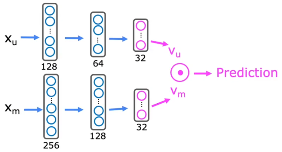
Cost Function: J = ∑ ( i , j ) : r ( i , j ) = 1 ( v u ( j ) ⋅ v m ( i ) − y ( i , j ) ) 2 + NN regularization term \text{Cost Function:}\quad J = \sum_{(i,j):\;r(i,j)=1}(v_u^{(j)}\cdot v_m^{(i)}-y^{(i,j)})^2 \textcolor{orange}{+\text{NN regularization term}} Cost Function:J=(i,j):r(i,j)=1∑(vu(j)⋅vm(i)−y(i,j))2+NN regularization term
- 假设 x ⃗ u ( j ) \vec{x}_u^{(j)} xu(j)长度为128、 v u ( j ) v_u^{(j)} vu(j)长度为32; x ⃗ m ( i ) \vec{x}_m^{(i)} xm(i)长度为256、 v m ( i ) v_m^{(i)} vm(i)长度为32。
上述就体现了神经网络“可连接性好”的优点,也就是可以很容易的将多个神经网络连接在一起进行训练。在实际的商业应用中,研究人员会精心挑选“原始特征” x ⃗ u ( j ) \vec{x}_u^{(j)} xu(j)、 x ⃗ m ( i ) \vec{x}_m^{(i)} xm(i),尽管这很耗时间,但是最后可以确保算法的性能良好。
3.2 从大型目录中推荐
在打开电影或者购物网站时,会在几秒之内就从数万甚至数百万个项目中,找到用户的“推荐内容”。即使神经网络已经预先训练完成,也不可能这么短的时间内全部计算完毕。实际上,当用户打开网站时,服务器只是检索最后的 v ⃗ u ( j ) \vec{v}_u^{(j)} vu(j)、 v ⃗ m ( i ) \vec{v}_m^{(i)} vm(i) 并计算了“向量点积”,其他都是预先计算好,下面就来介绍如何实现这种机制:
“检索(retrieval)”
- 生成候选项目列表,这个列表将尽可能涵盖用户所有可能感兴趣的内容。方法有:
- 根据用户最后观看的10部影片,然后找出和这10部电影最相似的10部电影。
- 根据用户最喜爱的前3种电影类型,找出这3种类型中最受欢迎的10部电影。
- 当前国家或地区最受欢迎的20部电影。
- 移除重复项、用户已经看过的电影,最后生成一个列表,比如长度为100。
注1:显然“项目列表”的长度越长,推荐结果越精确,但速度越慢。一般需要offline测试,来优化“性能-速度”的折衷。
注2:这可以提前计算 电影 k k k 和 电影 i i i 的相似程度: ∥ v ⃗ m ( k ) − v ⃗ m ( i ) ∥ 2 \lVert \vec{v}_m^{(k)}-\vec{v}_m^{(i)} \rVert^2 ∥vm(k)−vm(i)∥2,需要寻找相似电影时可以直接查表。“排名(ranking)”
- 将列表中的所有电影特征 v ⃗ m ( i ) \vec{v}_m^{(i)} vm(i) 和用户特征 v u ( j ) v_u^{(j)} vu(j) 进行点积,得到用户 j j j 对于每个电影所对应的预测评分 y ^ ( i , j ) \hat{y}^{(i,j)} y^(i,j)。
- 排序后展示给用户。
注:用户特征 v ⃗ u ( j ) \vec{v}_u^{(j)} vu(j) 一般都会提前计算出,用户登录时可以直接查表。
于是,按照上述流程,“基于内容过滤”的很大一部分工作都可以提前做好,于是每次用户点开网页时,主要的计算量是最后的“点积”运算,所以可以很快地完成“为你推荐”。
3.3 基于内容过滤的TensorFlow实现
在实际部署“基于内容过滤”的神经网络时,注意在进行向量相乘前,需要进行向量“长度归一化”。下面是代码框架:
import tensorflow as tf
# 定义用户特征的神经网络及输入输出
user_NN = tf.keras.models.Sequential([
    tf.keras.layers.Dense(256, activation='relu'),
    tf.keras.layers.Dense(128, activation='relu'),
    tf.keras.layers.Dense(32)
])
input_user = tf.keras.layers.Input(shape=(num_user_features))
vu = user_NN(input_user)                # 神经网络输入
vu = tf.linalg.l2_normalize(vu, axis=1) # 输出归一化

# 定义项目特征的神经网络及输入输出
item_NN = tf.keras.models.Sequential([
    tf.keras.layers.Dense(256, activation='relu'),
    tf.keras.layers.Dense(128, activation='relu'),
    tf.keras.layers.Dense(32)
])
input_item = tf.keras.layers.Input(shape=(num_item_features))
vm = item_NN(input_item)                # 神经网络输入
vm = tf.linalg.l2_normalize(vm, axis=1) # 输出归一化

# 将两个神经网络的输出进行点积
output = tf.keras.layers.Dot(axes=1)([vu, vm])

# 将上述两个网络合并,定义网络整体的输入输出
model = Model([input_user, input_item], output)

# 设置代价函数为平方误差
cost_fn = tf.keras.losses.MeanSquaredError()
3.4 推荐系统中的伦理
- 本节推荐视频:B站UP主“一只甜药”的“系统崩盘,算法作恶,互联网大厂怎么了?”
“基于内容过滤”的原理很快便介绍完了。本小节我们来讨论一些“推荐系统”的道德规范。显然,不同“推荐系统”的目标不同,有时候不得不在“公司利益”和“用户体验”之间做出一些妥协:
- 【合理】用户最喜欢的电影/体验。比如下左图,“旅游博主”既能分享自己的体验,也能挣到钱。
- 【合理】用户最可能购买的产品。
- 【质疑】用户最可能点击的广告。但是也会将广告费高的放在前面。
- 【质疑】可以为公司带来最大利益的产品。比如下右图,贷款公司倾向于“诱人贷款消费”。
- 【质疑】使用户的游玩时间/观看时间最长。更多推荐阴谋论/仇恨等极端言论。

于是,有时候“推荐系统”也会成为有害业务的放大器。下面是两种可能的解决方法:
- 加强监管,拒绝存在“剥削性业务”的公司所提供的广告。但这显然很难。
- 将算法的“推荐机制”透明公开,保护消费者知情权。
“推荐系统”是一个很强大的工具,老师希望我们在构建“推荐系统”时,也要思考可能会对社会产生的有害影响,我们的目标应该是让人类社会变得更好。
3.5 代码示例-基于内容过滤
本小节使用真实的电影评分数据集,来训练“基于内容过滤”的神经网络。最后自定义一个新用户特征,预测其感兴趣的电影。问题要求和代码结构如下:
问题要求:数据集给出了用户特征 x ⃗ u ( j ) \vec{x}_u^{(j)} xu(j)、电影特征 x ⃗ m ( i ) \vec{x}_m^{(i)} xm(i)、匹配结果 y ( i , j ) y^{(i,j)} y(i,j),将该数据集进行二拆分完成“基于内容过滤”训练,输出测试集性能并使用其预测新用户的偏好。
代码结构:
- 函数:若干,后续再补充注释。
- 主函数:加载原始数据集,然后对原始数据集进行“特征缩放(Course1-Week2-2.1节)”、二拆分,然后定义并训练“基于内容过滤”的神经网络,最后进行新用户预测。
注:本实验来自本周的练习“C3_W2_RecSysNN_Assignment.ipynb”。
注2:数据集见UP主提供的“课程资料”或者直接从百度网盘下载“C3-W2-3-5data(192KB)”。
The data set is derived from the MovieLens ml-latest-small dataset.
[F. Maxwell Harper and Joseph A. Konstan. 2015. The MovieLens Datasets: History and Context. ACM Transactions on Interactive Intelligent Systems (TiiS) 5, 4: 19:1–19:19. https://doi.org/10.1145/2827872]
下面是代码和运行结果:
import numpy as np
import numpy.ma as ma
from numpy import genfromtxt
from collections import defaultdict
import pandas as pd
pd.set_option("display.precision", 1)
import tensorflow as tf
from tensorflow import keras
from keras.models import Model
from sklearn.preprocessing import StandardScaler, MinMaxScaler
from sklearn.model_selection import train_test_split
import tabulate
import pickle
import csv
import re
######################################################################################
def load_data():
folder_path = 'C:/Users/14751/Desktop/机器学习-吴恩达/学习笔记'
item_train = genfromtxt(folder_path+'/data/content_item_train.csv', delimiter=',')
user_train = genfromtxt(folder_path+'/data/content_user_train.csv', delimiter=',')
y_train = genfromtxt(folder_path+'/data/content_y_train.csv', delimiter=',')
with open(folder_path+'/data/content_item_train_header.txt', newline='') as f: #csv reader handles quoted strings better
item_features = list(csv.reader(f))[0]
with open(folder_path+'/data/content_user_train_header.txt', newline='') as f:
user_features = list(csv.reader(f))[0]
item_vecs = genfromtxt(folder_path+'/data/content_item_vecs.csv', delimiter=',')
movie_dict = defaultdict(dict)
count = 0
with open(folder_path+'/data/content_movie_list.csv', newline='') as csvfile:
reader = csv.reader(csvfile, delimiter=',', quotechar='"')
for line in reader:
if count == 0:
count +=1 #skip header
#print(line)
else:
count +=1
movie_id = int(line[0])
movie_dict[movie_id]["title"] = line[1]
movie_dict[movie_id]["genres"] =line[2]
with open(folder_path+'/data/content_user_to_genre.pickle', 'rb') as f:
user_to_genre = pickle.load(f)
return(item_train, user_train, y_train, item_features, user_features, item_vecs, movie_dict, user_to_genre)
def pprint_train(x_train, features, vs, u_s, maxcount = 5, user=True):
""" Prints user_train or item_train nicely """
if user:
flist = [".0f",".0f",".1f",
".1f", ".1f", ".1f", ".1f",".1f",".1f", ".1f",".1f",".1f", ".1f",".1f",".1f",".1f",".1f"]
else:
flist = [".0f",".0f",".1f",
".0f",".0f",".0f", ".0f",".0f",".0f", ".0f",".0f",".0f", ".0f",".0f",".0f",".0f",".0f"]
head = features[:vs]
if vs < u_s: print("error, vector start {vs} should be greater then user start {u_s}")
for i in range(u_s):
head[i] = "[" + head[i] + "]"
genres = features[vs:]
hdr = head + genres
disp = [split_str(hdr, 5)]
count = 0
for i in range(0,x_train.shape[0]):
if count == maxcount: break
count += 1
disp.append( [
x_train[i,0].astype(int),
x_train[i,1].astype(int),
x_train[i,2].astype(float),
*x_train[i,3:].astype(float)
])
table = tabulate.tabulate(disp, tablefmt='html',headers="firstrow", floatfmt=flist, numalign='center')
return(table)
def pprint_data(y_p, user_train, item_train, printfull=False):
np.set_printoptions(precision=1)
for i in range(0,1000):
#print(f"{y_p[i,0]: 0.2f}, {ynorm_train.numpy()[i].item(): 0.2f}")
print(f"{
y_pu[i,0]: 0.2f}, {
y_train[i]: 0.2f}, ", end='')
print(f"{
user_train[i,0].astype(int):d}, ", end='') # userid
print(f"{
user_train[i,1].astype(int):d}, ", end=''), # rating cnt
print(f"{
user_train[i,2].astype(float): 0.2f}, ", end='') # rating ave
print(": ", end = '')
print(f"{
item_train[i,0].astype(int):d}, ", end='') # movie id
print(f"{
item_train[i,2].astype(float):0.1f}, ", end='') # ave movie rating
if printfull:
for j in range(8, user_train.shape[1]):
print(f"{
user_train[i,j].astype(float):0.1f}, ", end='') # rating
print(":", end='')
for j in range(3, item_train.shape[1]):
print(f"{
item_train[i,j].astype(int):d}, ", end='') # rating
print()
else:
a = user_train[i, uvs:user_train.shape[1]]
b = item_train[i, ivs:item_train.shape[1]]
c = np.multiply(a,b)
print(c)
def split_str(ifeatures, smax):
ofeatures = []
for s in ifeatures:
if ' ' not in s: # skip string that already have a space
if len(s) > smax:
mid = int(len(s)/2)
s = s[:mid] + " " + s[mid:]
ofeatures.append(s)
return(ofeatures)
def pprint_data_tab(y_p, user_train, item_train, uvs, ivs, user_features, item_features, maxcount = 20, printfull=False):
flist = [".1f", ".1f", ".0f", ".1f", ".0f", ".0f", ".0f",
".1f",".1f",".1f",".1f",".1f",".1f",".1f",".1f",".1f",".1f",".1f",".1f",".1f",".1f"]
user_head = user_features[:uvs]
genres = user_features[uvs:]
item_head = item_features[:ivs]
hdr = ["y_p", "y"] + user_head + item_head + genres
disp = [split_str(hdr, 5)]
count = 0
for i in range(0,y_p.shape[0]):
if count == maxcount: break
count += 1
a = user_train[i, uvs:user_train.shape[1]]
b = item_train[i, ivs:item_train.shape[1]]
c = np.multiply(a,b)
disp.append( [ y_p[i,0], y_train[i],
user_train[i,0].astype(int), # user id
user_train[i,1].astype(int), # rating cnt
user_train[i,2].astype(float), # user rating ave
item_train[i,0].astype(int), # movie id
item_train[i,1].astype(int), # year
item_train[i,2].astype(float), # ave movie rating
*c
])
table = tabulate.tabulate(disp, tablefmt='html',headers="firstrow", floatfmt=flist, numalign='center')
return(table)
def print_pred_movies(y_p, user, item, movie_dict, maxcount=10):
""" print results of prediction of a new user. inputs are expected to be in
sorted order, unscaled. """
count = 0
movies_listed = defaultdict(int)
disp = [["y_p", "movie id", "rating ave", "title", "genres"]]
for i in range(0, y_p.shape[0]):
if count == maxcount:
break
count += 1
movie_id = item[i, 0].astype(int)
if movie_id in movies_listed:
continue
movies_listed[movie_id] = 1
disp.append([y_p[i, 0], item[i, 0].astype(int), item[i, 2].astype(float),
movie_dict[movie_id]['title'], movie_dict[movie_id]['genres']])
table = tabulate.tabulate(disp, tablefmt='html',headers="firstrow")
return(table)
def gen_user_vecs(user_vec, num_items):
""" given a user vector return:
user predict maxtrix to match the size of item_vecs """
user_vecs = np.tile(user_vec, (num_items, 1))
return(user_vecs)
# predict on everything, filter on print/use
def predict_uservec(user_vecs, item_vecs, model, u_s, i_s, scaler, ScalerUser, ScalerItem, scaledata=False):
""" given a user vector, does the prediction on all movies in item_vecs returns
an array predictions sorted by predicted rating,
arrays of user and item, sorted by predicted rating sorting index
"""
if scaledata:
scaled_user_vecs = ScalerUser.transform(user_vecs)
scaled_item_vecs = ScalerItem.transform(item_vecs)
y_p = model.predict([scaled_user_vecs[:, u_s:], scaled_item_vecs[:, i_s:]])
else:
y_p = model.predict([user_vecs[:, u_s:], item_vecs[:, i_s:]])
y_pu = scaler.inverse_transform(y_p)
if np.any(y_pu < 0) :
print("Error, expected all positive predictions")
sorted_index = np.argsort(-y_pu,axis=0).reshape(-1).tolist() #negate to get largest rating first
sorted_ypu = y_pu[sorted_index]
sorted_items = item_vecs[sorted_index]
sorted_user = user_vecs[sorted_index]
return(sorted_index, sorted_ypu, sorted_items, sorted_user)
def print_pred_debug(y_p, y, user, item, maxcount=10, onlyrating=False, printfull=False):
""" hopefully reusable print. Keep for debug """
count = 0
for i in range(0, y_p.shape[0]):
if onlyrating == False or (onlyrating == True and y[i,0] != 0):
if count == maxcount: break
count += 1
print(f"{
y_p[i, 0]: 0.2f}, {
y[i,0]: 0.2f}, ", end='')
print(f"{
user[i, 0].astype(int):d}, ", end='') # userid
print(f"{
user[i, 1].astype(int):d}, ", end=''), # rating cnt
print(f"{
user[i, 2].astype(float):0.1f}, ", end=''), # rating ave
print(": ", end = '')
print(f"{
item[i, 0].astype(int):d}, ", end='') # movie id
print(f"{
item[i, 2].astype(float):0.1f}, ", end='') # ave movie rating
print(": ", end = '')
if printfull:
for j in range(uvs, user.shape[1]):
print(f"{
user[i, j].astype(float):0.1f}, ", end='') # rating
print(":", end='')
for j in range(ivs, item.shape[1]):
print(f"{
item[i, j].astype(int):d}, ", end='') # rating
print()
else:
a = user[i, uvs:user.shape[1]]
b = item[i, ivs:item.shape[1]]
c = np.multiply(a,b)
print(c)
def get_user_vecs(user_id, user_train, item_vecs, user_to_genre):
""" given a user_id, return:
user train/predict matrix to match the size of item_vecs
y vector with ratings for all rated movies and 0 for others of size item_vecs """
if user_id not in user_to_genre:
print("error: unknown user id")
return(None)
else:
user_vec_found = False
for i in range(len(user_train)):
if user_train[i, 0] == user_id:
user_vec = user_train[i]
user_vec_found = True
break
if not user_vec_found:
print("error in get_user_vecs, did not find uid in user_train")
num_items = len(item_vecs)
user_vecs = np.tile(user_vec, (num_items, 1))
y = np.zeros(num_items)
for i in range(num_items): # walk through movies in item_vecs and get the movies, see if user has rated them
movie_id = item_vecs[i, 0]
if movie_id in user_to_genre[user_id]['movies']:
rating = user_to_genre[user_id]['movies'][movie_id]
else:
rating = 0
y[i] = rating
return(user_vecs, y)
def get_item_genre(item, ivs, item_features):
offset = np.where(item[ivs:] == 1)[0][0]
genre = item_features[ivs + offset]
return(genre, offset)
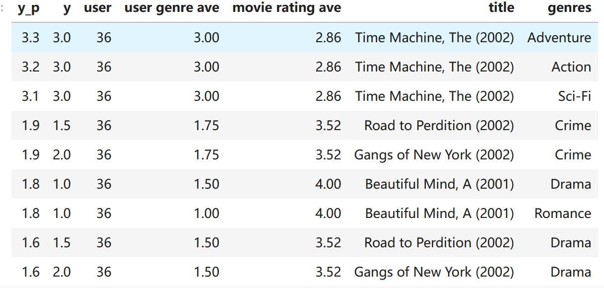
def print_existing_user(y_p, y, user, items, item_features, ivs, uvs, movie_dict, maxcount=10):
""" print results of prediction a user who was in the datatbase. inputs are expected to be in sorted order, unscaled. """
count = 0
movies_listed = defaultdict(int)
disp = [["y_p", "y", "user", "user genre ave", "movie rating ave", "title", "genres"]]
listed = []
count = 0
for i in range(0, y.shape[0]):
if y[i, 0] != 0:
if count == maxcount:
break
count += 1
movie_id = items[i, 0].astype(int)
offset = np.where(items[i, ivs:] == 1)[0][0]
genre_rating = user[i, uvs + offset]
genre = item_features[ivs + offset]
disp.append([y_p[i, 0], y[i, 0],
user[i, 0].astype(int), # userid
genre_rating.astype(float),
items[i, 2].astype(float), # movie average rating
movie_dict[movie_id]['title'], genre])
table = tabulate.tabulate(disp, tablefmt='html', headers="firstrow", floatfmt=[".1f", ".1f", ".0f", ".2f", ".2f"])
return(table)
######################################主函数##########################################
# 加载原始数据集
item_train, user_train, y_train, item_features, user_features, item_vecs, movie_dict, user_to_genre = load_data()
num_user_features = user_train.shape[1] - 3 # remove userid, rating count and ave rating during training
num_item_features = item_train.shape[1] - 1 # remove movie id at train time
uvs = 3 # user genre vector start
ivs = 3 # item genre vector start
u_s = 3 # start of columns to use in training, user
i_s = 1 # start of columns to use in training, items
scaledata = True # applies the standard scalar to data if true
print(f"用户特征x_u长度: {
num_user_features}")
print(f"电影特征x_m长度: {
num_item_features}")
print(f"数据集样本总数: {
len(item_train)}")
# 特征缩放:将数据转换为均值为0、方差为1的标准正态分布
print("\n对训练集进行缩放:")
if scaledata:
# 存储原始数据
item_train_ori = item_train
user_train_ori = user_train
# 项目特征缩放
scalerItem = StandardScaler()
scalerItem.fit(item_train)
item_train = scalerItem.transform(item_train)
# 用户特征缩放
scalerUser = StandardScaler()
scalerUser.fit(user_train)
user_train = scalerUser.transform(user_train)
# 将缩放后的特征逆变换观察是否匹配
print("电影特征item_train缩放成功?",np.allclose(item_train_ori, scalerItem.inverse_transform(item_train)))
print("用户特征user_train缩放成功?",np.allclose(user_train_ori, scalerUser.inverse_transform(user_train)))
# 神经网络输出结果缩放:将数据缩放到-1~1之间
y_train_ori = y_train # 保存原始数据
scalerY = MinMaxScaler((-1, 1))
scalerY.fit(y_train.reshape(-1, 1))
ynorm_train = scalerY.transform(y_train.reshape(-1, 1))
print("输出结果y_train缩放成功?",np.allclose(y_train, scalerY.inverse_transform(ynorm_train.reshape(1, -1))))
# 拆分原始数据集:训练集80%、测试集20%
item_train, item_test = train_test_split(item_train, train_size=0.80, shuffle=True, random_state=1)
user_train, user_test = train_test_split(user_train, train_size=0.80, shuffle=True, random_state=1)
ynorm_train, ynorm_test = train_test_split(ynorm_train, train_size=0.80, shuffle=True, random_state=1)
print(f"\n拆分原始数据集:训练集80%、测试集20%")
print(f"训练集大小: {
item_train.shape[0]}")
print(f"测试集大小: {
item_test.shape[0]}")
# 定义基于内容过滤的神经网络
num_outputs = 32
# tf.random.set_seed(1)
# 定义用户特征的神经网络及输入输出
user_NN = tf.keras.models.Sequential([
tf.keras.layers.Dense(256, activation='relu'),
tf.keras.layers.Dense(128, activation='relu'),
tf.keras.layers.Dense(num_outputs)
])
input_user = tf.keras.layers.Input(shape=(num_user_features))
vu = user_NN(input_user)
vu = tf.linalg.l2_normalize(vu, axis=1)
# 定义项目特征的神经网络及输入输出
item_NN = tf.keras.models.Sequential([
tf.keras.layers.Dense(256, activation='relu'),
tf.keras.layers.Dense(128, activation='relu'),
tf.keras.layers.Dense(num_outputs)
])
input_item = tf.keras.layers.Input(shape=(num_item_features))
vm = item_NN(input_item)
vm = tf.linalg.l2_normalize(vm, axis=1)
# 将两个神经网络的输出vu、vm进行点积
output = tf.keras.layers.Dot(axes=1)([vu, vm])
# 将上述两个网络合并,定义网络整体的输入输出
model = Model([input_user, input_item], output)
print(f"\n神经网络结构:")
print(f"v_u、v_m的长度为:{
num_outputs}")
model.summary()
# 使用训练集训练神经网络,并使用测试集评估性能
tf.random.set_seed(1)
cost_fn = tf.keras.losses.MeanSquaredError()
opt = keras.optimizers.Adam(learning_rate=0.01)
model.compile(optimizer=opt, loss=cost_fn, metrics='accuracy')
# tf.random.set_seed(1)
model.fit([user_train[:, u_s:], item_train[:, i_s:]], ynorm_train, epochs=30)
print('\n评估神经网络性能:')
model.evaluate([user_test[:, u_s:], item_test[:, i_s:]], ynorm_test)
# 下面来进行预测
# 定义新的用户特征向量x_u
new_user_id = 5000
new_rating_ave = 1.0
new_action = 1.0
new_adventure = 1
new_animation = 1
new_childrens = 1
new_comedy = 5
new_crime = 1
new_documentary = 1
new_drama = 1
new_fantasy = 1
new_horror = 1
new_mystery = 1
new_romance = 5
new_scifi = 5
new_thriller = 1
new_rating_count = 3
user_vec = np.array([[new_user_id, new_rating_count, new_rating_ave,
new_action, new_adventure, new_animation, new_childrens,
new_comedy, new_crime, new_documentary,
new_drama, new_fantasy, new_horror, new_mystery,
new_romance, new_scifi, new_thriller]])
# generate and replicate the user vector to match the number movies in the data set.
print(len(item_vecs))
user_vecs = gen_user_vecs(user_vec,len(item_vecs))
# scale the vectors and make predictions for all movies. Return results sorted by rating.
print("\n预测新用户的偏好:")
sorted_index, sorted_ypu, sorted_items, sorted_user = predict_uservec(
user_vecs, item_vecs, model, u_s, i_s,
scalerY, scalerUser, scalerItem, scaledata=scaledata)
print_pred_movies(sorted_ypu, sorted_user, sorted_items, movie_dict, maxcount = 10)
用户特征x_u长度: 14
电影特征x_m长度: 16
数据集样本总数: 58187

对训练集进行缩放:
电影特征item_train缩放成功? True
用户特征user_train缩放成功? True
输出结果y_train缩放成功? True

拆分原始数据集:训练集80%、测试集20%
训练集大小: 46549
测试集大小: 11638
WARNING:tensorflow:From D:\anaconda3\Lib\site-packages\keras\src\backend.py:873: The name tf.get_default_graph is deprecated. Please use tf.compat.v1.get_default_graph instead.

2023-12-15 10:40:43.839766: I tensorflow/core/platform/cpu_feature_guard.cc:182] This TensorFlow binary is optimized to use available CPU instructions in performance-critical operations.
To enable the following instructions: SSE SSE2 SSE3 SSE4.1 SSE4.2 AVX2 FMA, in other operations, rebuild TensorFlow with the appropriate compiler flags.

神经网络结构:
v_u、v_m的长度为:32
Model: "model"
__________________________________________________________________________________________________
 Layer (type)                Output Shape                 Param #   Connected to
==================================================================================================
 input_1 (InputLayer)        [(None, 14)]                 0         []

 input_2 (InputLayer)        [(None, 16)]                 0         []

 sequential (Sequential)     (None, 32)                   40864     ['input_1[0][0]']

 sequential_1 (Sequential)   (None, 32)                   41376     ['input_2[0][0]']

 tf.math.l2_normalize (TFOp  (None, 32)                   0         ['sequential[0][0]']
 Lambda)

 tf.math.l2_normalize_1 (TF  (None, 32)                   0         ['sequential_1[0][0]']
 OpLambda)

 dot (Dot)                   (None, 1)                    0         ['tf.math.l2_normalize[0][0]',
                                                                     'tf.math.l2_normalize_1[0][0]
                                                                    ']

==================================================================================================
Total params: 82240 (321.25 KB)
Trainable params: 82240 (321.25 KB)
Non-trainable params: 0 (0.00 Byte)
__________________________________________________________________________________________________
Epoch 1/30
WARNING:tensorflow:From D:\anaconda3\Lib\site-packages\keras\src\utils\tf_utils.py:492: The name tf.ragged.RaggedTensorValue is deprecated. Please use tf.compat.v1.ragged.RaggedTensorValue instead.

WARNING:tensorflow:From D:\anaconda3\Lib\site-packages\keras\src\engine\base_layer_utils.py:384: The name tf.executing_eagerly_outside_functions is deprecated. Please use tf.compat.v1.executing_eagerly_outside_functions instead.

1455/1455 [==============================] - 3s 1ms/step - loss: 0.1252 - accuracy: 0.0753
Epoch 2/30
1455/1455 [==============================] - 2s 1ms/step - loss: 0.1182 - accuracy: 0.0792
Epoch 3/30
1455/1455 [==============================] - 2s 1ms/step - loss: 0.1167 - accuracy: 0.0791
Epoch 4/30
1455/1455 [==============================] - 2s 1ms/step - loss: 0.1148 - accuracy: 0.0796
Epoch 5/30
1455/1455 [==============================] - 2s 1ms/step - loss: 0.1135 - accuracy: 0.0812
Epoch 6/30
1455/1455 [==============================] - 2s 1ms/step - loss: 0.1123 - accuracy: 0.0801
Epoch 7/30
1455/1455 [==============================] - 2s 1ms/step - loss: 0.1116 - accuracy: 0.0805
Epoch 8/30
1455/1455 [==============================] - 2s 1ms/step - loss: 0.1108 - accuracy: 0.0809
Epoch 9/30
1455/1455 [==============================] - 2s 1ms/step - loss: 0.1097 - accuracy: 0.0819
Epoch 10/30
1455/1455 [==============================] - 2s 1ms/step - loss: 0.1084 - accuracy: 0.0822
Epoch 11/30
1455/1455 [==============================] - 2s 1ms/step - loss: 0.1071 - accuracy: 0.0824
Epoch 12/30
1455/1455 [==============================] - 2s 1ms/step - loss: 0.1068 - accuracy: 0.0828
Epoch 13/30
1455/1455 [==============================] - 3s 2ms/step - loss: 0.1060 - accuracy: 0.0832
Epoch 14/30
1455/1455 [==============================] - 3s 2ms/step - loss: 0.1052 - accuracy: 0.0835
Epoch 15/30
1455/1455 [==============================] - 2s 1ms/step - loss: 0.1045 - accuracy: 0.0836
Epoch 16/30
1455/1455 [==============================] - 2s 1ms/step - loss: 0.1038 - accuracy: 0.0840
Epoch 17/30
1455/1455 [==============================] - 2s 1ms/step - loss: 0.1032 - accuracy: 0.0837
Epoch 18/30
1455/1455 [==============================] - 2s 2ms/step - loss: 0.1028 - accuracy: 0.0838
Epoch 19/30
1455/1455 [==============================] - 2s 1ms/step - loss: 0.1021 - accuracy: 0.0843
Epoch 20/30
1455/1455 [==============================] - 2s 1ms/step - loss: 0.1017 - accuracy: 0.0851
Epoch 21/30
1455/1455 [==============================] - 2s 1ms/step - loss: 0.1011 - accuracy: 0.0848
Epoch 22/30
1455/1455 [==============================] - 2s 1ms/step - loss: 0.1006 - accuracy: 0.0851
Epoch 23/30
1455/1455 [==============================] - 2s 1ms/step - loss: 0.1000 - accuracy: 0.0861
Epoch 24/30
1455/1455 [==============================] - 2s 1ms/step - loss: 0.0996 - accuracy: 0.0857
Epoch 25/30
1455/1455 [==============================] - 2s 1ms/step - loss: 0.0992 - accuracy: 0.0856
Epoch 26/30
1455/1455 [==============================] - 2s 1ms/step - loss: 0.0986 - accuracy: 0.0863
Epoch 27/30
1455/1455 [==============================] - 2s 1ms/step - loss: 0.0983 - accuracy: 0.0861
Epoch 28/30
1455/1455 [==============================] - 2s 1ms/step - loss: 0.0980 - accuracy: 0.0865
Epoch 29/30
1455/1455 [==============================] - 2s 1ms/step - loss: 0.0974 - accuracy: 0.0860
Epoch 30/30
1455/1455 [==============================] - 2s 1ms/step - loss: 0.0971 - accuracy: 0.0861

评估神经网络性能:
364/364 [==============================] - 0s 762us/step - loss: 0.1042 - accuracy: 0.0861
1883

预测新用户的偏好:
59/59 [==============================] - 0s 765us/step
本节 Quiz:
Vector x ⃗ u \vec{x}_u xu and vector x ⃗ m \vec{x}_m xm must be of the same dimension, where x ⃗ u \vec{x}_u xu is the input features vector for a user (age, gender, etc.). x ⃗ m \vec{x}_m xm is the input features vector for a movie (year, genre, etc.). True or false?
False:可以不是一个维度If we find that two movies, i i i and k k k, have vectors v ⃗ m ( i ) \vec{v}_m^{(i)} vm(i) and v ⃗ m ( k ) \vec{v}_m^{(k)} vm(k) that are similar to each other(i.e., ∥ v ⃗ m ( i ) − v ⃗ m ( k ) ∥ \lVert \vec{v}_m^{(i)} - \vec{v}_m^{(k)} \rVert ∥vm(i)−vm(k)∥ is small), then which of the following is likely to be true? Pick the best answer.
√ The two movies are similar to each other and will be liked by similar users.
× The two movies are very dissimilar.
× We should recommend to users one of these two movies, but not both.
× A user that has watched one of these two movies has probably watched the other as well.Which of the following neural network configurations are valid for a content based filtering application? Please note carefully the dimensions of the neural network indicated in the diagram. Check all the options that apply:
√ Both the user and the item networks have the same architecture.
√ The user and the item networks have different architectures.
× The user vector v ⃗ u \vec{v}_u vu is 32 dimensional, and the item vector v ⃗ m \vec{v}_m vm is 64 dimensional.
√ The user and item networks have 64 dimensional v ⃗ u \vec{v}_u vu and v ⃗ m \vec{v}_m vm vector respectively.You have built a recommendation system to retrieve musical pieces from a large database of music, and have an algorithm that uses separate retrieval and ranking steps. If you modify the algorithm to add more musical pieces to the retrieved list (i.e., the retrieval step returns more items), which of these are likely to happen? Check all that apply.
√ The system’s response time might increase (i.e, users have to wait longer to get recommendations).
× The quality of recommendations made to users should stay the same or worsen.
× The system’s response time might decrease (i.e, users get recommendations more quickly).
√ The quality of recommendations made to users should stay the same or improve.To speed up the response time of your recommendation system, you can pre-compute the vectors v ⃗ m \vec{v}_m vm for all the items you might recommend. This can be done even before a user logs in to your website and even before you know the x ⃗ u \vec{x}_u xu or v ⃗ u \vec{v}_u vu vector. True/False?
√ True
× False
4. 主成分分析(选修)
“主成分分析(Principal Component Analysis, PCA)”是一个经常用于可视化的“无监督学习”算法,其主要的应用领域有:
- 【常用】数据可视化:将高维数据(比如50维、1000维等)压缩成二维、三维,以进行绘图及可视化。并且也可以将压缩后数据恢复成原始数据。
- 【没落】数据压缩:显然上述“数据可视化”的过程就是“数据压缩”。但随着存储和网络的发展,对于压缩需求变小,并且也有更先进的数据压缩算法,所以此应用逐渐没落。
- 【没落】加速有监督学习:先将数据集的原始特征进行压缩,再进行“有监督学习”(如“支持向量机SVM”)。但对于现在的深度学习来说,压缩原始特征并没有太大帮助,并且PCA本身也会消耗计算资源,所以此应用逐渐没落。
下面就来介绍如何使用PCA算法进行“数据可视化”。
4.1 PCA算法原理
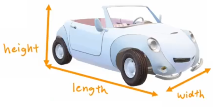
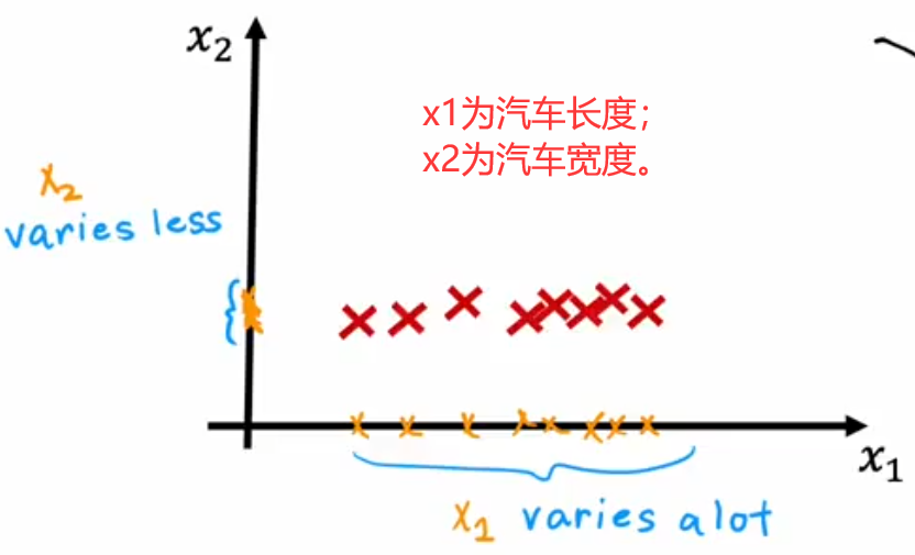

- 长度和宽度: x 1 x_1 x1表示汽车长度、 x 2 x_2 x2表示汽车宽度。由于道路宽度限制, x 2 x_2 x2变化不多,所以可以直接将汽车长度 ( x 1 x_1 x1轴) 作为压缩后的特征。
- 长度和高度: x 1 x_1 x1表示汽车长度、 x 2 x_2 x2表示汽车高度。我们可以定义一个新的“z轴”,使用各个样本点投影到“z轴”的长度来作为压缩后的特征。
PCA算法的思想是找到一组新轴,来最大可能的表示出样本间的差异。如上图所示,就展示了两个压缩二维汽车数据的示例。那该如何寻找这个具有代表性的“z轴”呢?答案是最大化方差。假设n维原始数据集为 m × n m\times n m×n 的二维矩阵 X X X,每一行都代表一个样本 x ⃗ ( i ) \vec{x}^{(i)} x(i),于是PCA算法的具体步骤如下:
- 均值归一化。计算所有样本的均值 μ ⃗ \vec{\mu} μ,然后每个样本都减去此均值: x ⃗ n ( i ) = x ⃗ ( i ) − μ ⃗ \vec{x}^{(i)}_n = \vec{x}^{(i)}-\vec{\mu} xn(i)=x(i)−μ (下标 n n n强调“均值归一化”)。
- 选取“主成分轴”。过原点旋转z轴,z轴的单位方向向量为 z ⃗ n 1 \vec{z}_{n}^1 zn1 (下标 n n n强调“单位向量”),然后根据所有样本在当前z轴的投影 x ⃗ n ( i ) ⋅ z ⃗ n 1 \vec{x}^{(i)}_n\cdot\vec{z}_n^1 xn(i)⋅zn1 计算方差,方差最大的就是“主成分轴”。
- 选取剩余轴。z轴确定后,剩余其他轴都依次成90°,并计算出单位方向向量 z ⃗ n 2 \vec{z}_{n}^2 zn2、 z ⃗ n 3 \vec{z}_{n}^3 zn3(可视化一般不超过3维)。
- 计算样本新坐标。新坐标就是在各轴上的投影: [ x ⃗ n ( i ) ⋅ z ⃗ n 1 , x ⃗ n ( i ) ⋅ z ⃗ n 2 , x ⃗ n ( i ) ⋅ z ⃗ n 3 ] [\vec{x}^{(i)}_n\cdot\vec{z}_n^1, \;\; \vec{x}^{(i)}_n\cdot\vec{z}_n^2, \;\; \vec{x}^{(i)}_n\cdot\vec{z}_n^3] [xn(i)⋅zn1,xn(i)⋅zn2,xn(i)⋅zn3]。
注:“均值归一化”是为了可以“过原点”旋转z轴,所以“均值归一化”很关键。
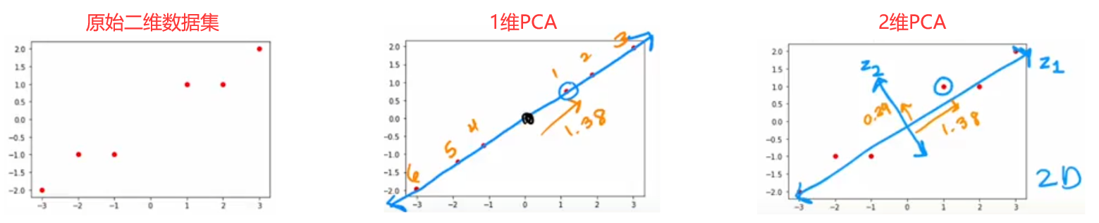
注:下图给出了使用PCA计算“投影”,以及根据新坐标长度“重构(reconstration)”出原始坐标的方法。

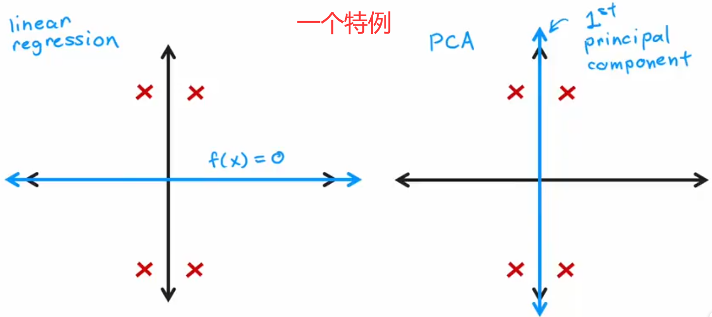
最后要说明一点,“PCA算法”不是“线性回归”,两者的差别很大:
- 线性回归是“有监督学习”;PCA算法是“无监督学习”。
- 线性回归“最小化平方误差”;PCA算法“最大化方差”。
- 线性回归是为了“预测”;PCA算法只是为了减少特征数量,方便可视化。
注:下右图使用一个特例,展示了两者的区别。

4.2 PCA算法的代码实现
在Python中,主要使用 scikit-learn库来实现PCA。下面是两个代码示例:
- 使用PCA将2维数据压缩成2维数据,只是为了展示压缩后新坐标轴相互垂直。
from sklearn.decomposition import PCA
import numpy as np
######################## 将2维数据压缩成1维 #########################
X = np.array([[1,1], [2,1], [3,2], [-1,-1], [-2,-1], [-3,-2]])
pca_1 = PCA(n_components=1)                     # 设置压缩后维度
pca_1.fit(X)                                    # PCA压缩维度
print(pca_1.explained_variance_ratio_)          # 0.992
X_trans_1 = pca_1.transform(X)                  # 计算压缩后坐标(投影)
X_reduced_1 = pca.inverse_transform(X_trans_1)  # 重构
# X_trans_1 : array([
#             [ 1.38340578] ,
#             [ 2.22189802] ,
#             [ 3.6053038 ] ,
#             [-1.38340578] ,
#             [-2.22189802] ,
#             [-3.6053038 ]])
######################## 将2维数据压缩成2维 #########################
X = np.array([[1,1], [2,1], [3,2], [-1,-1], [-2,-1], [-3,-2]])
pca_2 = PCA(n_components=2)                     # 设置压缩后维度
pca_2.fit(X)                                    # PCA压缩维度
print(pca_2.explained_variance_ratio_)          # [0.992, 0.008]
X_trans_2 = pca_2.transform(X)                  # 计算压缩后坐标(投影)
X_reduced_2 = pca.inverse_transform(X_trans_2)  # 重构
# X_trans_2 : array([
#             [ 1.38340578,  0.2935787 ] ,
#             [ 2.22189802, -0.25133484] ,
#             [ 3.6053038 ,  0.04224385] ,
#             [-1.38340578, -0.2935787 ] ,
#             [-2.22189802,  0.25133484] ,
#             [-3.6053038 , -0.04224385])
智能推荐
python编码问题之encode、decode、codecs模块_python中encode在什么模块-程序员宅基地
文章浏览阅读2.1k次。原文链接先说说编解码问题编码转换时,通常需要以unicode作为中间编码,即先将其他编码的字符串解码(decode)成unicode,再从unicode编码(encode)成另一种编码。 Eg:str1.decode('gb2312') #将gb2312编码的字符串转换成unicode编码str2.encode('gb2312') #将unicode编码..._python中encode在什么模块
Java数据流-程序员宅基地
文章浏览阅读949次,点赞21次,收藏15次。本文介绍了Java中的数据输入流(DataInputStream)和数据输出流(DataOutputStream)的使用方法。
ie浏览器无法兼容的问题汇总_ie 浏览器 newdate-程序员宅基地
文章浏览阅读111次。ie无法兼容_ie 浏览器 newdate
想用K8s,还得先会Docker吗?其实完全没必要-程序员宅基地
文章浏览阅读239次。这篇文章把 Docker 和 K8s 的关系给大家做了一个解答,希望还在迟疑自己现有的知识储备能不能直接学 K8s 的,赶紧行动起来,K8s 是典型的入门有点难,后面越用越香。
ADI中文手册获取方法_adi 如何查看数据手册-程序员宅基地
文章浏览阅读561次。ADI中文手册获取方法_adi 如何查看数据手册
React 分页-程序员宅基地
文章浏览阅读1k次,点赞4次,收藏3次。React 获取接口数据实现分页效果以拼多多接口为例实现思路加载前 加载动画加载后 判断有内容的时候 无内容的时候用到的知识点1、动画效果(用在加载前,加载之后就隐藏或关闭,用开关效果即可)2、axios请求3、map渲染页面4、分页插件(antd)代码实现import React, { Component } from 'react';//引入axiosimport axios from 'axios';//引入antd插件import { Pagination }_react 分页
随便推点
关于使用CryPtopp库进行RSA签名与验签的一些说明_cryptopp 签名-程序员宅基地
文章浏览阅读449次,点赞9次,收藏7次。这个变量与验签过程中的SignatureVerificationFilter::PUT_MESSAGE这个宏是对应的,SignatureVerificationFilter::PUT_MESSAGE,如果在签名过程中putMessage设置为true,则在验签过程中需要添加SignatureVerificationFilter::PUT_MESSAGE。项目中使用到了CryPtopp库进行RSA签名与验签,但是在使用过程中反复提示无效的数字签名。否则就会出现文章开头出现的数字签名无效。_cryptopp 签名
新闻稿的写作格式_新闻稿时间应该放在什么位置-程序员宅基地
文章浏览阅读848次。新闻稿是新闻从业者经常使用的一种文体,它的格式与内容都有着一定的规范。本文将从新闻稿的格式和范文两个方面进行介绍,以帮助读者更好地了解新闻稿的写作_新闻稿时间应该放在什么位置
Java中的转换器设计模式_java转换器模式-程序员宅基地
文章浏览阅读1.7k次。Java中的转换器设计模式 在这篇文章中,我们将讨论 Java / J2EE项目中最常用的 Converter Design Pattern。由于Java8 功能不仅提供了相应类型之间的通用双向转换方式,而且还提供了转换相同类型对象集合的常用方法,从而将样板代码减少到绝对最小值。我们使用Java8 功能编写了..._java转换器模式
应用k8s入门-程序员宅基地
文章浏览阅读150次。1,kubectl run创建pods[root@master ~]# kubectl run nginx-deploy --image=nginx:1.14-alpine --port=80 --replicas=1[root@master ~]# kubectl get podsNAME READY STATUS REST...
PAT菜鸡进化史_乙级_1003_1003 pat乙级 最优-程序员宅基地
文章浏览阅读128次。PAT菜鸡进化史_乙级_1003“答案正确”是自动判题系统给出的最令人欢喜的回复。本题属于 PAT 的“答案正确”大派送 —— 只要读入的字符串满足下列条件,系统就输出“答案正确”,否则输出“答案错误”。得到“答案正确”的条件是: 1. 字符串中必须仅有 P、 A、 T这三种字符,不可以包含其它字符; 2. 任意形如 xPATx 的字符串都可以获得“答案正确”,其中 x 或者是空字符串,或..._1003 pat乙级 最优
CH340与Android串口通信_340串口小板 安卓给安卓发指令-程序员宅基地
文章浏览阅读5.6k次。CH340与Android串口通信为何要将CH340的ATD+Eclipse上的安卓工程移植到AndroidStudio移植的具体步骤CH340串口通信驱动函数通信过程中重难点还存在的问题为何要将CH340的ATD+Eclipse上的安卓工程移植到AndroidStudio为了在这个工程基础上进行改动,验证串口的数据和配置串口的参数,我首先在Eclipse上配置了安卓开发环境,注意在配置环境是..._340串口小板 安卓给安卓发指令