【六 (2)机器学习-EDA探索性数据分析模板】-程序员宅基地
技术标签: 简明数据分析进阶路径 python 数据分析 机器学习 人工智能
目录
文章导航
一、EDA:
EDA(Exploratory Data Analysis)即探索性数据分析,EDA通过可视化、统计和图形化的方法,对数据集进行全面的、非形式化的初步分析,帮助分析人员了解数据的基本特征,发现数据中的规律和模式。这有助于获取对数据的直观感受和深刻理解,为后续的数据处理和建模提供基础。
二、导入类库
# 导入类库
import numpy as np
import pandas as pd
import scipy.stats as stats

import matplotlib.pyplot as plt
import seaborn as sns
import plotly.express as px

import warnings
warnings.filterwarnings('ignore')
from sklearn.preprocessing import LabelEncoder
from sklearn.preprocessing import RobustScaler

from sklearn.decomposition import PCA
from sklearn.model_selection import cross_val_score, GridSearchCV, KFold

from sklearn.base import BaseEstimator, TransformerMixin, RegressorMixin
from sklearn.base import clone
from sklearn.linear_model import Lasso
from sklearn.linear_model import LinearRegression
from sklearn.linear_model import Ridge
from sklearn.ensemble import RandomForestRegressor, GradientBoostingRegressor, ExtraTreesRegressor
from sklearn.svm import SVR, LinearSVR
from sklearn.linear_model import ElasticNet, SGDRegressor, BayesianRidge
from sklearn.kernel_ridge import KernelRidge
from xgboost import XGBRegressor
# 显示中文
plt.rcParams['font.sans-serif'] = ['SimHei']
plt.rcParams['axes.unicode_minus'] = False

# pandas显示所有行和列
pd.set_option('display.max_columns', None)
pd.set_option('display.max_rows', None)
三、导入数据
train = pd.read_csv('./train.csv')
test = pd.read_csv('./test.csv')

train.head()
四、查看数据类型和缺失情况
train.info()
<class 'pandas.core.frame.DataFrame'>
RangeIndex: 90615 entries, 0 to 90614
Data columns (total 10 columns):
 #   Column          Non-Null Count  Dtype
---  ------          --------------  -----
 0   id              90615 non-null  int64
 1   Sex             90615 non-null  object
 2   Length          90615 non-null  float64
 3   Diameter        90615 non-null  float64
 4   Height          90615 non-null  float64
 5   Whole weight    90615 non-null  float64
 6   Whole weight.1  90615 non-null  float64
 7   Whole weight.2  90615 non-null  float64
 8   Shell weight    90615 non-null  float64
 9   Rings           90615 non-null  int64
dtypes: float64(7), int64(2), object(1)
memory usage: 6.9+ MB
五、确认目标变量和ID
Target_features = ['Rings'] #目标变量
ID_features = ['id'] #id
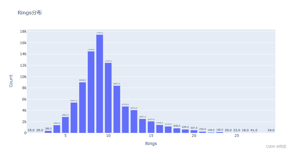
六、查看目标变量分布情况
Target_counts = train[Target_features].value_counts().reset_index()
Target_counts.columns = [Target_features[0], 'Count']


# 绘制条形图
fig = px.bar(Target_counts,x=Target_features[0], y='Count', title=Target_features[0]+'分布')

# 遍历每个轨迹并设置文本
def set_text(trace):
    trace.text = [f"{val:.1f}" for val in trace.y]
    trace.textposition = 'outside'

fig.for_each_trace(set_text)

# 显示图表
fig.show()
七、特征变量按照数据类型分成定量变量和定性变量
# 移除ID和目标变量
train_columns = list(train.columns)
train_columns.remove(Target_features[0])
train_columns.remove(ID_features[0])

# 特征变量按照数据类型分成定量变量和定性变量
quantitative = [feature for feature in train_columns if train.dtypes[feature] != 'object'] # 定量变量
print('定量变量')
print(quantitative)
qualitative = [feature for feature in train_columns if train.dtypes[feature] == 'object'] # 定性变量
print('定性变量')
print(qualitative)
定量变量
['Length', 'Diameter', 'Height', 'Whole weight', 'Whole weight.1', 'Whole weight.2', 'Shell weight']
定性变量
['Sex']
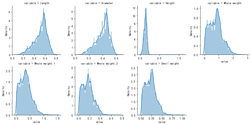
八、查看定量变量分布情况
# 查看定量变量分布情况
m_cont = pd.melt(train, value_vars=quantitative)
g = sns.FacetGrid(m_cont, col='variable', col_wrap=4, sharex=False, sharey=False)
g.map(sns.distplot, 'value')
九、查看定量变量的离散程度
# 查看定量变量的离散程度
def plot_boxplots(df):
    m_disc = pd.melt(df)
    g = sns.FacetGrid(m_disc, col='variable', col_wrap=4, sharex=False, sharey=False)
    g.map(sns.boxplot, 'variable', 'value', width=0.5)
    plt.show()

plot_boxplots(train[quantitative])

十、查看定量变量与目标变量关系
# 定量变量与目标变量关系图
m_cont = pd.melt(train, id_vars=Target_features[0], value_vars=quantitative)
g = sns.FacetGrid(m_cont, col='variable', col_wrap=4, sharex=False, sharey=True)
g.map(plt.scatter, 'value', Target_features[0])

十一、查看定性变量分布情况
# 定性变量频数统计图
m_disc = pd.melt(train, value_vars=qualitative)
g = sns.FacetGrid(m_disc, col='variable', col_wrap=4, sharex=False, sharey=False)
g.map(sns.countplot, 'value')

十二、查看定性变量与目标变量关系
# 定性变量与目标变量关系图
m_disc = pd.melt(train, id_vars=Target_features[0], value_vars=qualitative)
g = sns.FacetGrid(m_disc, col='variable', col_wrap=4, sharex=False, sharey=False)
g.map(sns.boxplot, 'value', Target_features[0])

十三、查看定性变量对目标变量的显著性影响
# 查看定性变量对目标变量的显著性影响
def anova(frame, qualitative):
    anv = pd.DataFrame()
    anv['feature'] = qualitative
    p_vals = []
    for fea in qualitative:
        samples = []
        cls = frame[fea].unique() # 变量的类别值
        for c in cls:
            c_array = frame[frame[fea]==c][Target_features[0]].values
            samples.append(c_array)
        p_val = stats.f_oneway(*samples)[1] # 获得p值,p值越小,对SalePrice的显著性影响越大
        p_vals.append(p_val)
    anv['pval'] = p_vals
    return anv.sort_values('pval')
a = anova(train, qualitative)
a['disparity'] = np.log(1./a['pval'].values) # 对SalePrice的影响悬殊度
plt.figure(figsize=(8, 6))
sns.barplot(x='feature', y='disparity', data=a)
plt.xticks(rotation=90)
plt.show()

十四、查看定性变量和目标变量的spearman相关系数
# 查看定性变量和目标变量的spearman相关系数
# 需要先把定性变量处理为数值类型
def encode(frame, feature):
    ordering = pd.DataFrame()
    ordering['val'] = frame[feature].unique()
    ordering.index = ordering['val']
    ordering['spmean'] = frame[[feature, Target_features[0]]].groupby(feature)[Target_features[0]].mean()
    ordering = ordering.sort_values('spmean')
    ordering['ordering'] = np.arange(1, ordering.shape[0]+1)
    ordering = ordering['ordering'].to_dict() # 返回的数据样例{category1:1, category2:2, ...}

    # 对frame[feature]编码
    for category, code_value in ordering.items():
        frame.loc[frame[feature]==category, feature+'_E'] = code_value
qual_encoded = []
for qual in qualitative:
    encode(train, qual)
    qual_encoded.append(qual+'_E')
# print(qual_encoded)

def spearman(frame, features):
    spr =  pd.DataFrame()
    spr['feature'] = features
    spr['spearman'] = [frame[f].corr(frame[Target_features[0]], 'spearman') for f in features]
    spr = spr.sort_values('spearman')

    plt.figure(figsize=(6, 0.25*len(features)))
    sns.barplot(x='spearman', y='feature', data=spr)
spearman(train, quantitative+qual_encoded)

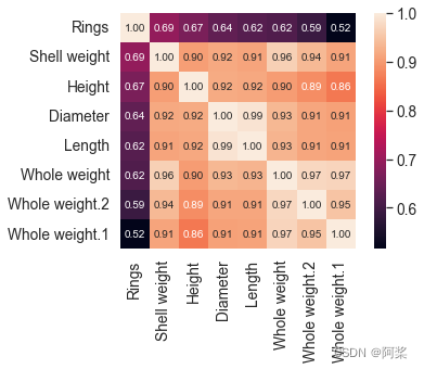
十五、查看定量变量与目标变量相关性
# 定量变量与目标变量相关性
# plt.figure(1, figsize=(12,9))
corrmat = train[quantitative+[Target_features[0]]].corr()
k = 10 #number of variables for heatmap
cols = corrmat.nlargest(k, Target_features[0])[Target_features[0]].index
corr = train[list(cols)].corr()
sns.set(font_scale=1.25)
sns.heatmap(corr, cbar=True, annot=True, square=True, fmt='.2f', annot_kws={'size': 10}, yticklabels=cols.values, xticklabels=cols.values)
plt.show()
十六、查看定性变量与目标变量相关性
# 定性变量与目标变量相关性

# plt.figure(1, figsize=(12,9))
corrmat = train[qual_encoded+[Target_features[0]]].corr()
k = 10 #number of variables for heatmap
cols = corrmat.nlargest(k, Target_features[0])[Target_features[0]].index
corr = train[list(cols)].corr()
sns.set(font_scale=1.25)
sns.heatmap(corr, cbar=True, annot=True, square=True, fmt='.2f', annot_kws={'size': 10}, yticklabels=cols.values, xticklabels=cols.values)
plt.show()

智能推荐
攻防世界_难度8_happy_puzzle_攻防世界困难模式攻略图文-程序员宅基地
文章浏览阅读645次。这个肯定是末尾的IDAT了,因为IDAT必须要满了才会开始一下个IDAT,这个明显就是末尾的IDAT了。,对应下面的create_head()代码。,对应下面的create_tail()代码。不要考虑爆破,我已经试了一下,太多情况了。题目来源:UNCTF。_攻防世界困难模式攻略图文
达梦数据库的导出(备份)、导入_达梦数据库导入导出-程序员宅基地
文章浏览阅读2.9k次,点赞3次,收藏10次。偶尔会用到,记录、分享。1. 数据库导出1.1 切换到dmdba用户su - dmdba1.2 进入达梦数据库安装路径的bin目录,执行导库操作 导出语句:./dexp cwy_init/[email protected]:5236 file=cwy_init.dmp log=cwy_init_exp.log 注释: cwy_init/init_123..._达梦数据库导入导出
js引入kindeditor富文本编辑器的使用_kindeditor.js-程序员宅基地
文章浏览阅读1.9k次。1. 在官网上下载KindEditor文件,可以删掉不需要要到的jsp,asp,asp.net和php文件夹。接着把文件夹放到项目文件目录下。2. 修改html文件,在页面引入js文件:<script type="text/javascript" src="./kindeditor/kindeditor-all.js"></script><script type="text/javascript" src="./kindeditor/lang/zh-CN.js"_kindeditor.js
STM32学习过程记录11——基于STM32G431CBU6硬件SPI+DMA的高效WS2812B控制方法-程序员宅基地
文章浏览阅读2.3k次,点赞6次,收藏14次。SPI的详情简介不必赘述。假设我们通过SPI发送0xAA,我们的数据线就会变为10101010,通过修改不同的内容,即可修改SPI中0和1的持续时间。比如0xF0即为前半周期为高电平,后半周期为低电平的状态。在SPI的通信模式中,CPHA配置会影响该实验,下图展示了不同采样位置的SPI时序图[1]。CPOL = 0,CPHA = 1:CLK空闲状态 = 低电平,数据在下降沿采样,并在上升沿移出CPOL = 0,CPHA = 0:CLK空闲状态 = 低电平,数据在上升沿采样,并在下降沿移出。_stm32g431cbu6
计算机网络-数据链路层_接收方收到链路层数据后,使用crc检验后,余数为0,说明链路层的传输时可靠传输-程序员宅基地
文章浏览阅读1.2k次,点赞2次,收藏8次。数据链路层习题自测问题1.数据链路(即逻辑链路)与链路(即物理链路)有何区别?“电路接通了”与”数据链路接通了”的区别何在?2.数据链路层中的链路控制包括哪些功能?试讨论数据链路层做成可靠的链路层有哪些优点和缺点。3.网络适配器的作用是什么?网络适配器工作在哪一层?4.数据链路层的三个基本问题(帧定界、透明传输和差错检测)为什么都必须加以解决?5.如果在数据链路层不进行帧定界,会发生什么问题?6.PPP协议的主要特点是什么?为什么PPP不使用帧的编号?PPP适用于什么情况?为什么PPP协议不_接收方收到链路层数据后,使用crc检验后,余数为0,说明链路层的传输时可靠传输
软件测试工程师移民加拿大_无证移民,未受过软件工程师的教育(第1部分)-程序员宅基地
文章浏览阅读587次。软件测试工程师移民加拿大 无证移民,未受过软件工程师的教育(第1部分) (Undocumented Immigrant With No Education to Software Engineer(Part 1))Before I start, I want you to please bear with me on the way I write, I have very little gen...
随便推点
Thinkpad X250 secure boot failed 启动失败问题解决_安装完系统提示secureboot failure-程序员宅基地
文章浏览阅读304次。Thinkpad X250笔记本电脑,装的是FreeBSD,进入BIOS修改虚拟化配置(其后可能是误设置了安全开机),保存退出后系统无法启动,显示:secure boot failed ,把自己惊出一身冷汗,因为这台笔记本刚好还没开始做备份.....根据错误提示,到bios里面去找相关配置,在Security里面找到了Secure Boot选项,发现果然被设置为Enabled,将其修改为Disabled ,再开机,终于正常启动了。_安装完系统提示secureboot failure
C++如何做字符串分割(5种方法)_c++ 字符串分割-程序员宅基地
文章浏览阅读10w+次,点赞93次,收藏352次。1、用strtok函数进行字符串分割原型: char *strtok(char *str, const char *delim);功能:分解字符串为一组字符串。参数说明:str为要分解的字符串,delim为分隔符字符串。返回值:从str开头开始的一个个被分割的串。当没有被分割的串时则返回NULL。其它:strtok函数线程不安全,可以使用strtok_r替代。示例://借助strtok实现split#include <string.h>#include <stdio.h&_c++ 字符串分割
2013第四届蓝桥杯 C/C++本科A组 真题答案解析_2013年第四届c a组蓝桥杯省赛真题解答-程序员宅基地
文章浏览阅读2.3k次。1 .高斯日记 大数学家高斯有个好习惯:无论如何都要记日记。他的日记有个与众不同的地方,他从不注明年月日,而是用一个整数代替,比如:4210后来人们知道,那个整数就是日期,它表示那一天是高斯出生后的第几天。这或许也是个好习惯,它时时刻刻提醒着主人:日子又过去一天,还有多少时光可以用于浪费呢?高斯出生于:1777年4月30日。在高斯发现的一个重要定理的日记_2013年第四届c a组蓝桥杯省赛真题解答
基于供需算法优化的核极限学习机(KELM)分类算法-程序员宅基地
文章浏览阅读851次,点赞17次,收藏22次。摘要:本文利用供需算法对核极限学习机(KELM)进行优化,并用于分类。
metasploitable2渗透测试_metasploitable2怎么进入-程序员宅基地
文章浏览阅读1.1k次。一、系统弱密码登录1、在kali上执行命令行telnet 192.168.26.1292、Login和password都输入msfadmin3、登录成功,进入系统4、测试如下:二、MySQL弱密码登录:1、在kali上执行mysql –h 192.168.26.129 –u root2、登录成功,进入MySQL系统3、测试效果:三、PostgreSQL弱密码登录1、在Kali上执行psql -h 192.168.26.129 –U post..._metasploitable2怎么进入
Python学习之路:从入门到精通的指南_python人工智能开发从入门到精通pdf-程序员宅基地
文章浏览阅读257次。本文将为初学者提供Python学习的详细指南,从Python的历史、基础语法和数据类型到面向对象编程、模块和库的使用。通过本文,您将能够掌握Python编程的核心概念,为今后的编程学习和实践打下坚实基础。_python人工智能开发从入门到精通pdf