TensorFlow图像分类:如何构建分类器-程序员宅基地
导言
图像分类对于我们来说是一件非常容易的事情,但是对于一台机器来说,在人工智能和深度学习广泛使用之前,这是一项艰巨的任务。自动驾驶汽车能够实时检测物体并采取相应必要的行动,并且由于TensorFlow图像分类,大部分都可以实现。
在本文中,将你共同学习以下内容:
什么是TensorFlow?
什么是图像分类?
TensorFlow图像分类:Fashion-MNIST
CIFAR 10:CNN
什么是TensorFlow?
TensorFlow是Google的开源机器学习框架,用于跨越一些列任务进行数据流编程。图中的节点表示数学运算,而图表边表示在它们之间传递的多维数据阵列。
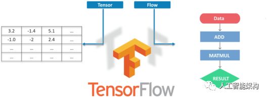
Tensors是多维数组,是二维表到具有更高维度的数据的扩展。TensorFlow的许多功能使其适合深度学习,它的核心开源库可以帮助大家开发和训练ML模型。
什么是图像分类?
图像分类的目的是将数字图像中的所有像素分类为若干类或主题之一。然后,该分类数据可用于显示图像中的物体是否存在与以上分类或主题。

根据分类过程中的交互,有两种类型的分类:
监督
无监督
所以,我们直接通过两个例子学习TensorFlow图像分类。
TensorFlow图像分类:Fashion-MNIST
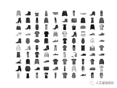
Fashion-MNIST数据集
在这里,我们将使用Fashion MNIST Dataset,它包含10个类别中的70,000个灰度图像。我们将使用60,000个进行训练,10,000个进行测试。如果你想自己尝试,可以直接从TensorFlow访问Fashion MNIST,导入并加载数据即可。
导入库
1from __future__ import absolute_import, division, print_function2# TensorFlow and tf.keras3import tensorflow as tf4from tensorflow import keras5# Helper libraries6import numpy as np7import matplotlib.pyplot as pltimport absolute_import, division, print_function
2# TensorFlow and tf.keras
3import tensorflow as tf
4from tensorflow import keras
5# Helper libraries
6import numpy as np
7import matplotlib.pyplot as plt
加载数据
1fashion_mnist = keras.datasets.fashion_mnist2(train_images, train_labels), (test_images, test_labels) = fashion_mnist.load_data()
2(train_images, train_labels), (test_images, test_labels) = fashion_mnist.load_data()
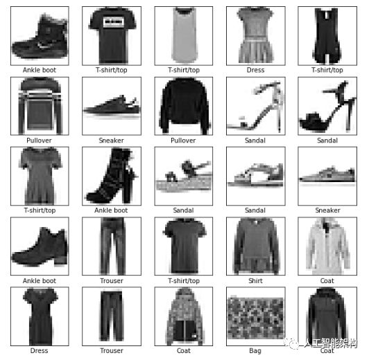
将把图像映射到类中
1class_names = ['T-shirt/top', 'Trouser', 'Pullover', 'Dress', 'Coat','Sandal', 'Shirt', 'Sneaker', 'Bag', 'Ankle boot']'T-shirt/top', 'Trouser', 'Pullover', 'Dress', 'Coat','Sandal', 'Shirt', 'Sneaker', 'Bag', 'Ankle boot']
探索数据
1train_images.shape2#Each Label is between 0-93train_labels4test_images.shape
2#Each Label is between 0-9
3train_labels
4test_images.shape
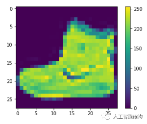
预处理数据
1plt.figure()2plt.imshow(train_images[0])3plt.colorbar()4plt.grid(False)5plt.show()6#If you inspect the first image in the training set, you will see that the pixel values fall in the range of 0 to 255.
2plt.imshow(train_images[0])
3plt.colorbar()
4plt.grid(False)
5plt.show()
6#If you inspect the first image in the training set, you will see that the pixel values fall in the range of 0 to 255.
缩放0-1图像,将其输入神经网络
1train_images = train_images / 255.02test_images = test_images / 255.0255.0
2test_images = test_images / 255.0
显示部分图像
 1plt.figure(figsize=(10,10)) 2for i in range(25): 3    plt.subplot(5,5,i+1) 4    plt.xticks([]) 5    plt.yticks([]) 6    plt.grid(False) 7    plt.imshow(train_images[i], cmap=plt.cm.binary) 8    plt.xlabel(class_names[train_labels[i]]) 9plt.show()1010,10))
 2for i in range(25):
 3    plt.subplot(5,5,i+1)
 4    plt.xticks([])
 5    plt.yticks([])
 6    plt.grid(False)
 7    plt.imshow(train_images[i], cmap=plt.cm.binary)
 8    plt.xlabel(class_names[train_labels[i]])
 9plt.show()
10
设置层
1model = keras.Sequential([2    keras.layers.Flatten(input_shape=(28, 28)),3    keras.layers.Dense(128, activation=tf.nn.relu),4    keras.layers.Dense(10, activation=tf.nn.softmax)5])
2    keras.layers.Flatten(input_shape=(28, 28)),
3    keras.layers.Dense(128, activation=tf.nn.relu),
4    keras.layers.Dense(10, activation=tf.nn.softmax)
5])
编译模型
1model.compile(optimizer='adam',2              loss='sparse_categorical_crossentropy',3              metrics=['accuracy'])'adam',
2              loss='sparse_categorical_crossentropy',
3              metrics=['accuracy'])
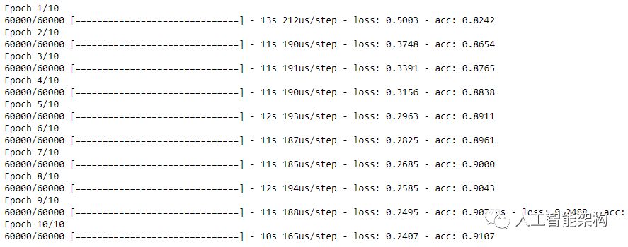
模型训练
1model.fit(train_images, train_labels, epochs=10)10)
评估准确性
1test_loss, test_acc = model.evaluate(test_images, test_labels)2print('Test accuracy:', test_acc)
2print('Test accuracy:', test_acc)

预测
1predictions = model.predict(test_images)2predictions[0]
2predictions[0]
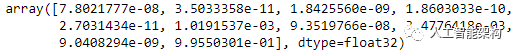
预测结果是10个数字的数组,即对应于图像的10种不同服装中的每一种。我们可以看到哪个标签具有最高的置信度值。
1np.argmax(predictions[0])2#Model is most confident that it's an ankle boot. Let's see if it's correct30])
2#Model is most confident that it's an ankle boot. Let's see if it's correct
3
输出:9
1test_labels[0]0]
查看10个全集
 1def plot_image(i, predictions_array, true_label, img): 2  predictions_array, true_label, img = predictions_array[i], true_label[i], img[i] 3  plt.grid(False) 4  plt.xticks([]) 5  plt.yticks([]) 6  plt.imshow(img, cmap=plt.cm.binary) 7  predicted_label = np.argmax(predictions_array) 8  if predicted_label == true_label: 9    color = 'green'10  else:11    color = 'red'12  plt.xlabel("{} {:2.0f}% ({})".format(class_names[predicted_label],13                                100*np.max(predictions_array),14                                class_names[true_label]),15                                color=color)16def plot_value_array(i, predictions_array, true_label):17  predictions_array, true_label = predictions_array[i], true_label[i]18  plt.grid(False)19  plt.xticks([])20  plt.yticks([])21  thisplot = plt.bar(range(10), predictions_array, color="#777777")22  plt.ylim([0, 1])23  predicted_label = np.argmax(predictions_array)24  thisplot[predicted_label].set_color('red')25  thisplot[true_label].set_color('green')def plot_image(i, predictions_array, true_label, img):
 2  predictions_array, true_label, img = predictions_array[i], true_label[i], img[i]
 3  plt.grid(False)
 4  plt.xticks([])
 5  plt.yticks([])
 6  plt.imshow(img, cmap=plt.cm.binary)
 7  predicted_label = np.argmax(predictions_array)
 8  if predicted_label == true_label:
 9    color = 'green'
10  else:
11    color = 'red'
12  plt.xlabel("{} {:2.0f}% ({})".format(class_names[predicted_label],
13                                100*np.max(predictions_array),
14                                class_names[true_label]),
15                                color=color)
16def plot_value_array(i, predictions_array, true_label):
17  predictions_array, true_label = predictions_array[i], true_label[i]
18  plt.grid(False)
19  plt.xticks([])
20  plt.yticks([])
21  thisplot = plt.bar(range(10), predictions_array, color="#777777")
22  plt.ylim([0, 1])
23  predicted_label = np.argmax(predictions_array)
24  thisplot[predicted_label].set_color('red')
25  thisplot[true_label].set_color('green')
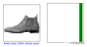
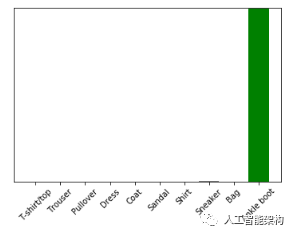
第0张和第10张图片
1i = 02plt.figure(figsize=(6,3))3plt.subplot(1,2,1)4plot_image(i, predictions, test_labels, test_images)5plt.subplot(1,2,2)6plot_value_array(i, predictions,  test_labels)7plt.show()0
2plt.figure(figsize=(6,3))
3plt.subplot(1,2,1)
4plot_image(i, predictions, test_labels, test_images)
5plt.subplot(1,2,2)
6plot_value_array(i, predictions,  test_labels)
7plt.show()
1i = 102plt.figure(figsize=(6,3))3plt.subplot(1,2,1)4plot_image(i, predictions, test_labels, test_images)5plt.subplot(1,2,2)6plot_value_array(i, predictions,  test_labels)7plt.show()10
2plt.figure(figsize=(6,3))
3plt.subplot(1,2,1)
4plot_image(i, predictions, test_labels, test_images)
5plt.subplot(1,2,2)
6plot_value_array(i, predictions,  test_labels)
7plt.show()
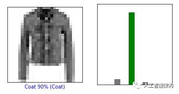
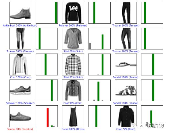
绘制几幅图像进行预测。正确为绿色,不正确为红色
 1num_rows = 5 2num_cols = 3 3num_images = num_rows*num_cols 4plt.figure(figsize=(2*2*num_cols, 2*num_rows)) 5for i in range(num_images): 6  plt.subplot(num_rows, 2*num_cols, 2*i+1) 7  plot_image(i, predictions, test_labels, test_images) 8  plt.subplot(num_rows, 2*num_cols, 2*i+2) 9  plot_value_array(i, predictions, test_labels)10plt.show()5
 2num_cols = 3
 3num_images = num_rows*num_cols
 4plt.figure(figsize=(2*2*num_cols, 2*num_rows))
 5for i in range(num_images):
 6  plt.subplot(num_rows, 2*num_cols, 2*i+1)
 7  plot_image(i, predictions, test_labels, test_images)
 8  plt.subplot(num_rows, 2*num_cols, 2*i+2)
 9  plot_value_array(i, predictions, test_labels)
10plt.show()
使用训练的模型对单个图像进行预测
 1# Grab an image from the test dataset 2img = test_images[0] 3 4print(img.shape) 5 6# Add the image to a batch where it's the only member. 7img = (np.expand_dims(img,0)) 8 9print(img.shape)1011predictions_single = model.predict(img) 12print(predictions_single)# Grab an image from the test dataset
 2img = test_images[0]
 3
 4print(img.shape)
 5
 6# Add the image to a batch where it's the only member.
 7img = (np.expand_dims(img,0))
 8
 9print(img.shape)
10
11predictions_single = model.predict(img)
12print(predictions_single)

1plot_value_array(0, predictions_single, test_labels)2plt.xticks(range(10), class_names, rotation=45)3plt.show()0, predictions_single, test_labels)
2plt.xticks(range(10), class_names, rotation=45)
3plt.show()
批量处理唯一图像的预测
1prediction_result = np.argmax(predictions_single[0])0])
CIFAR-10: CNN
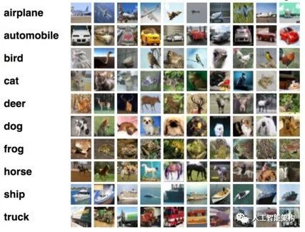
CIFAR-10数据集由飞机、狗、猫和其他物体组成。对图像进行预处理,然后在所有样本上训练卷积神经网络。需要对图像进行标准化。通过这个用例肯定能解释你曾经对TensorFlow图像分类的疑虑。
下载数据
 1from urllib.request import urlretrieve 2from os.path import isfile, isdir 3from tqdm import tqdm  4import tarfile 5cifar10_dataset_folder_path = 'cifar-10-batches-py' 6class DownloadProgress(tqdm): 7    last_block = 0 8    def hook(self, block_num=1, block_size=1, total_size=None): 9        self.total = total_size10        self.update((block_num - self.last_block) * block_size)11        self.last_block = block_num12""" 13    check if the data (zip) file is already downloaded14    if not, download it from "https://www.cs.toronto.edu/~kriz/cifar-10-python.tar.gz" and save as cifar-10-python.tar.gz15"""16if not isfile('cifar-10-python.tar.gz'):17    with DownloadProgress(unit='B', unit_scale=True, miniters=1, desc='CIFAR-10 Dataset') as pbar:18        urlretrieve(19            'https://www.cs.toronto.edu/~kriz/cifar-10-python.tar.gz',20            'cifar-10-python.tar.gz',21            pbar.hook)22if not isdir(cifar10_dataset_folder_path):23    with tarfile.open('cifar-10-python.tar.gz') as tar:24        tar.extractall()25        tar.close()from urllib.request import urlretrieve
 2from os.path import isfile, isdir
 3from tqdm import tqdm
 4import tarfile
 5cifar10_dataset_folder_path = 'cifar-10-batches-py'
 6class DownloadProgress(tqdm):
 7    last_block = 0
 8    def hook(self, block_num=1, block_size=1, total_size=None):
 9        self.total = total_size
10        self.update((block_num - self.last_block) * block_size)
11        self.last_block = block_num
12"""
13    check if the data (zip) file is already downloaded
14    if not, download it from "https://www.cs.toronto.edu/~kriz/cifar-10-python.tar.gz" and save as cifar-10-python.tar.gz
15"""
16if not isfile('cifar-10-python.tar.gz'):
17    with DownloadProgress(unit='B', unit_scale=True, miniters=1, desc='CIFAR-10 Dataset') as pbar:
18        urlretrieve(
19            'https://www.cs.toronto.edu/~kriz/cifar-10-python.tar.gz',
20            'cifar-10-python.tar.gz',
21            pbar.hook)
22if not isdir(cifar10_dataset_folder_path):
23    with tarfile.open('cifar-10-python.tar.gz') as tar:
24        tar.extractall()
25        tar.close()
导入必要的库
1import pickle2import numpy as np3import matplotlib.pyplot as pltimport pickle
2import numpy as np
3import matplotlib.pyplot as plt
了解数据
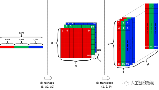
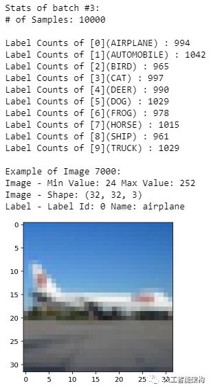
原始数据批量为10000*3072张,用numpy数组表示,其中10000是样本数据的数量。图像时彩色的,尺寸为32*32.可以(width x height x num_channel)或(num_channel x width x height)的格式进行输入。我们定义标签。
重塑数据
将分为两个阶段重塑数据。
首先,将行向量(3072)分成3个。每个部分对应于每个通道,维度将是3*1024.然后将上一步的结果除以32,这里的32是图像的宽度,则将为3*32*32.
其次,我们必须将数据从(num_channel,width,height)转置为(width,height,num_channel)。使用转置函数。
1def load_cfar10_batch(cifar10_dataset_folder_path, batch_id):2    with open(cifar10_dataset_folder_path + '/data_batch_' + str(batch_id), mode='rb') as file:3        # note the encoding type is 'latin1'4        batch = pickle.load(file, encoding='latin1')5    features = batch['data'].reshape((len(batch['data']), 3, 32, 32)).transpose(0, 2, 3, 1)6    labels = batch['labels']7    return features, labeldef load_cfar10_batch(cifar10_dataset_folder_path, batch_id):
2    with open(cifar10_dataset_folder_path + '/data_batch_' + str(batch_id), mode='rb') as file:
3        # note the encoding type is 'latin1'
4        batch = pickle.load(file, encoding='latin1')
5    features = batch['data'].reshape((len(batch['data']), 3, 32, 32)).transpose(0, 2, 3, 1)
6    labels = batch['labels']
7    return features, label
探索数据
1%matplotlib inline2%config InlineBackend.figure_format = 'retina'3import numpy as np4# Explore the dataset5batch_id = 36sample_id = 70007display_stats(cifar10_dataset_folder_path, batch_id, sample_id)
2%config InlineBackend.figure_format = 'retina'
3import numpy as np
4# Explore the dataset
5batch_id = 3
6sample_id = 7000
7display_stats(cifar10_dataset_folder_path, batch_id, sample_id)
实现预处理功能
通过Min-Max Normalization标准化数据。可以简单的是所有x值的范围在0和1之间。
y = (x-min) / (max-min)
编码
 1def one_hot_encode(x): 2    """ 3        argument 4            - x: a list of labels 5        return 6            - one hot encoding matrix (number of labels, number of class) 7    """ 8    encoded = np.zeros((len(x), 10)) 9    for idx, val in enumerate(x):10        encoded[idx][val] = 111    return encodeddef one_hot_encode(x):
 2    """
 3        argument
 4            - x: a list of labels
 5        return
 6            - one hot encoding matrix (number of labels, number of class)
 7    """
 8    encoded = np.zeros((len(x), 10))
 9    for idx, val in enumerate(x):
10        encoded[idx][val] = 1
11    return encoded
预处理和保存数据
 1def _preprocess_and_save(normalize, one_hot_encode, features, labels, filename): 2    features = normalize(features) 3    labels = one_hot_encode(labels) 4    pickle.dump((features, labels), open(filename, 'wb')) 5def preprocess_and_save_data(cifar10_dataset_folder_path, normalize, one_hot_encode): 6    n_batches = 5 7    valid_features = [] 8    valid_labels = [] 9    for batch_i in range(1, n_batches + 1):10        features, labels = load_cfar10_batch(cifar10_dataset_folder_path, batch_i)11        # find index to be the point as validation data in the whole dataset of the batch (10%)12        index_of_validation = int(len(features) * 0.1)13        # preprocess the 90% of the whole dataset of the batch14        # - normalize the features15        # - one_hot_encode the lables16        # - save in a new file named, "preprocess_batch_" + batch_number17        # - each file for each batch18        _preprocess_and_save(normalize, one_hot_encode,19                             features[:-index_of_validation], labels[:-index_of_validation], 20                             'preprocess_batch_' + str(batch_i) + '.p')21        # unlike the training dataset, validation dataset will be added through all batch dataset22        # - take 10% of the whold dataset of the batch23        # - add them into a list of24        #   - valid_features25        #   - valid_labels26        valid_features.extend(features[-index_of_validation:])27        valid_labels.extend(labels[-index_of_validation:])28    # preprocess the all stacked validation dataset29    _preprocess_and_save(normalize, one_hot_encode,30                         np.array(valid_features), np.array(valid_labels),31                         'preprocess_validation.p')32    # load the test dataset33    with open(cifar10_dataset_folder_path + '/test_batch', mode='rb') as file:34        batch = pickle.load(file, encoding='latin1')35    # preprocess the testing data36    test_features = batch['data'].reshape((len(batch['data']), 3, 32, 32)).transpose(0, 2, 3, 1)37    test_labels = batch['labels']38    # Preprocess and Save all testing data39    _preprocess_and_save(normalize, one_hot_encode,40                         np.array(test_features), np.array(test_labels),41                         'preprocess_training.p')def _preprocess_and_save(normalize, one_hot_encode, features, labels, filename):
 2    features = normalize(features)
 3    labels = one_hot_encode(labels)
 4    pickle.dump((features, labels), open(filename, 'wb'))
 5def preprocess_and_save_data(cifar10_dataset_folder_path, normalize, one_hot_encode):
 6    n_batches = 5
 7    valid_features = []
 8    valid_labels = []
 9    for batch_i in range(1, n_batches + 1):
10        features, labels = load_cfar10_batch(cifar10_dataset_folder_path, batch_i)
11        # find index to be the point as validation data in the whole dataset of the batch (10%)
12        index_of_validation = int(len(features) * 0.1)
13        # preprocess the 90% of the whole dataset of the batch
14        # - normalize the features
15        # - one_hot_encode the lables
16        # - save in a new file named, "preprocess_batch_" + batch_number
17        # - each file for each batch
18        _preprocess_and_save(normalize, one_hot_encode,
19                             features[:-index_of_validation], labels[:-index_of_validation],
20                             'preprocess_batch_' + str(batch_i) + '.p')
21        # unlike the training dataset, validation dataset will be added through all batch dataset
22        # - take 10% of the whold dataset of the batch
23        # - add them into a list of
24        #   - valid_features
25        #   - valid_labels
26        valid_features.extend(features[-index_of_validation:])
27        valid_labels.extend(labels[-index_of_validation:])
28    # preprocess the all stacked validation dataset
29    _preprocess_and_save(normalize, one_hot_encode,
30                         np.array(valid_features), np.array(valid_labels),
31                         'preprocess_validation.p')
32    # load the test dataset
33    with open(cifar10_dataset_folder_path + '/test_batch', mode='rb') as file:
34        batch = pickle.load(file, encoding='latin1')
35    # preprocess the testing data
36    test_features = batch['data'].reshape((len(batch['data']), 3, 32, 32)).transpose(0, 2, 3, 1)
37    test_labels = batch['labels']
38    # Preprocess and Save all testing data
39    _preprocess_and_save(normalize, one_hot_encode,
40                         np.array(test_features), np.array(test_labels),
41                         'preprocess_training.p')
建立网络
整个模型共有14层。

 1import tensorflow as tf 2def conv_net(x, keep_prob): 3    conv1_filter = tf.Variable(tf.truncated_normal(shape=[3, 3, 3, 64], mean=0, stddev=0.08)) 4    conv2_filter = tf.Variable(tf.truncated_normal(shape=[3, 3, 64, 128], mean=0, stddev=0.08)) 5    conv3_filter = tf.Variable(tf.truncated_normal(shape=[5, 5, 128, 256], mean=0, stddev=0.08)) 6    conv4_filter = tf.Variable(tf.truncated_normal(shape=[5, 5, 256, 512], mean=0, stddev=0.08)) 7    # 1, 2 8    conv1 = tf.nn.conv2d(x, conv1_filter, strides=[1,1,1,1], padding='SAME') 9    conv1 = tf.nn.relu(conv1)10    conv1_pool = tf.nn.max_pool(conv1, ksize=[1,2,2,1], strides=[1,2,2,1], padding='SAME')11    conv1_bn = tf.layers.batch_normalization(conv1_pool)12    # 3, 413    conv2 = tf.nn.conv2d(conv1_bn, conv2_filter, strides=[1,1,1,1], padding='SAME')14    conv2 = tf.nn.relu(conv2)15    conv2_pool = tf.nn.max_pool(conv2, ksize=[1,2,2,1], strides=[1,2,2,1], padding='SAME')    16    conv2_bn = tf.layers.batch_normalization(conv2_pool)17    # 5, 618    conv3 = tf.nn.conv2d(conv2_bn, conv3_filter, strides=[1,1,1,1], padding='SAME')19    conv3 = tf.nn.relu(conv3)20    conv3_pool = tf.nn.max_pool(conv3, ksize=[1,2,2,1], strides=[1,2,2,1], padding='SAME')  21    conv3_bn = tf.layers.batch_normalization(conv3_pool)22    # 7, 823    conv4 = tf.nn.conv2d(conv3_bn, conv4_filter, strides=[1,1,1,1], padding='SAME')24    conv4 = tf.nn.relu(conv4)25    conv4_pool = tf.nn.max_pool(conv4, ksize=[1,2,2,1], strides=[1,2,2,1], padding='SAME')26    conv4_bn = tf.layers.batch_normalization(conv4_pool)27    # 928    flat = tf.contrib.layers.flatten(conv4_bn)  29    # 1030    full1 = tf.contrib.layers.fully_connected(inputs=flat, num_outputs=128, activation_fn=tf.nn.relu)31    full1 = tf.nn.dropout(full1, keep_prob)32    full1 = tf.layers.batch_normalization(full1)33    # 1134    full2 = tf.contrib.layers.fully_connected(inputs=full1, num_outputs=256, activation_fn=tf.nn.relu)35    full2 = tf.nn.dropout(full2, keep_prob)36    full2 = tf.layers.batch_normalization(full2)37    # 1238    full3 = tf.contrib.layers.fully_connected(inputs=full2, num_outputs=512, activation_fn=tf.nn.relu)39    full3 = tf.nn.dropout(full3, keep_prob)40    full3 = tf.layers.batch_normalization(full3)    41    # 1342    full4 = tf.contrib.layers.fully_connected(inputs=full3, num_outputs=1024, activation_fn=tf.nn.relu)43    full4 = tf.nn.dropout(full4, keep_prob)44    full4 = tf.layers.batch_normalization(full4)        45    # 1446    out = tf.contrib.layers.fully_connected(inputs=full3, num_outputs=10, activation_fn=None)47    return outimport tensorflow as tf
 2def conv_net(x, keep_prob):
 3    conv1_filter = tf.Variable(tf.truncated_normal(shape=[3, 3, 3, 64], mean=0, stddev=0.08))
 4    conv2_filter = tf.Variable(tf.truncated_normal(shape=[3, 3, 64, 128], mean=0, stddev=0.08))
 5    conv3_filter = tf.Variable(tf.truncated_normal(shape=[5, 5, 128, 256], mean=0, stddev=0.08))
 6    conv4_filter = tf.Variable(tf.truncated_normal(shape=[5, 5, 256, 512], mean=0, stddev=0.08))
 7    # 1, 2
 8    conv1 = tf.nn.conv2d(x, conv1_filter, strides=[1,1,1,1], padding='SAME')
 9    conv1 = tf.nn.relu(conv1)
10    conv1_pool = tf.nn.max_pool(conv1, ksize=[1,2,2,1], strides=[1,2,2,1], padding='SAME')
11    conv1_bn = tf.layers.batch_normalization(conv1_pool)
12    # 3, 4
13    conv2 = tf.nn.conv2d(conv1_bn, conv2_filter, strides=[1,1,1,1], padding='SAME')
14    conv2 = tf.nn.relu(conv2)
15    conv2_pool = tf.nn.max_pool(conv2, ksize=[1,2,2,1], strides=[1,2,2,1], padding='SAME')
16    conv2_bn = tf.layers.batch_normalization(conv2_pool)
17    # 5, 6
18    conv3 = tf.nn.conv2d(conv2_bn, conv3_filter, strides=[1,1,1,1], padding='SAME')
19    conv3 = tf.nn.relu(conv3)
20    conv3_pool = tf.nn.max_pool(conv3, ksize=[1,2,2,1], strides=[1,2,2,1], padding='SAME')
21    conv3_bn = tf.layers.batch_normalization(conv3_pool)
22    # 7, 8
23    conv4 = tf.nn.conv2d(conv3_bn, conv4_filter, strides=[1,1,1,1], padding='SAME')
24    conv4 = tf.nn.relu(conv4)
25    conv4_pool = tf.nn.max_pool(conv4, ksize=[1,2,2,1], strides=[1,2,2,1], padding='SAME')
26    conv4_bn = tf.layers.batch_normalization(conv4_pool)
27    # 9
28    flat = tf.contrib.layers.flatten(conv4_bn)
29    # 10
30    full1 = tf.contrib.layers.fully_connected(inputs=flat, num_outputs=128, activation_fn=tf.nn.relu)
31    full1 = tf.nn.dropout(full1, keep_prob)
32    full1 = tf.layers.batch_normalization(full1)
33    # 11
34    full2 = tf.contrib.layers.fully_connected(inputs=full1, num_outputs=256, activation_fn=tf.nn.relu)
35    full2 = tf.nn.dropout(full2, keep_prob)
36    full2 = tf.layers.batch_normalization(full2)
37    # 12
38    full3 = tf.contrib.layers.fully_connected(inputs=full2, num_outputs=512, activation_fn=tf.nn.relu)
39    full3 = tf.nn.dropout(full3, keep_prob)
40    full3 = tf.layers.batch_normalization(full3)
41    # 13
42    full4 = tf.contrib.layers.fully_connected(inputs=full3, num_outputs=1024, activation_fn=tf.nn.relu)
43    full4 = tf.nn.dropout(full4, keep_prob)
44    full4 = tf.layers.batch_normalization(full4)
45    # 14
46    out = tf.contrib.layers.fully_connected(inputs=full3, num_outputs=10, activation_fn=None)
47    return out
超参数
1epochs = 102batch_size = 1283keep_probability = 0.74learning_rate = 0.00110
2batch_size = 128
3keep_probability = 0.7
4learning_rate = 0.001
1logits = conv_net(x, keep_prob)2model = tf.identity(logits, name='logits') # Name logits Tensor, so that can be loaded from disk after training3# Loss and Optimizer4cost = tf.reduce_mean(tf.nn.softmax_cross_entropy_with_logits(logits=logits, labels=y))5optimizer = tf.train.AdamOptimizer(learning_rate=learning_rate).minimize(cost)6# Accuracy7correct_pred = tf.equal(tf.argmax(logits, 1), tf.argmax(y, 1))8accuracy = tf.reduce_mean(tf.cast(correct_pred, tf.float32), name='accuracy')
2model = tf.identity(logits, name='logits') # Name logits Tensor, so that can be loaded from disk after training
3# Loss and Optimizer
4cost = tf.reduce_mean(tf.nn.softmax_cross_entropy_with_logits(logits=logits, labels=y))
5optimizer = tf.train.AdamOptimizer(learning_rate=learning_rate).minimize(cost)
6# Accuracy
7correct_pred = tf.equal(tf.argmax(logits, 1), tf.argmax(y, 1))
8accuracy = tf.reduce_mean(tf.cast(correct_pred, tf.float32), name='accuracy')
训练神经网络
1#Single Optimizationdef train_neural_network(session, optimizer, keep_probability, feature_batch, label_batch):2    session.run(optimizer, 3                feed_dict={4                    x: feature_batch,5                    y: label_batch,6                    keep_prob: keep_probability7                })#Single Optimizationdef train_neural_network(session, optimizer, keep_probability, feature_batch, label_batch):
2    session.run(optimizer,
3                feed_dict={

4                    x: feature_batch,
5                    y: label_batch,
6                    keep_prob: keep_probability
7                })
 1#Showing Stats 2def print_stats(session, feature_batch, label_batch, cost, accuracy): 3    loss = sess.run(cost,  4                    feed_dict={ 5                        x: feature_batch, 6                        y: label_batch, 7                        keep_prob: 1. 8                    }) 9    valid_acc = sess.run(accuracy, 10                         feed_dict={11                             x: valid_features,12                             y: valid_labels,13                             keep_prob: 1.14                         })15    print('Loss: {:>10.4f} Validation Accuracy: {:.6f}'.format(loss, valid_acc))#Showing Stats
 2def print_stats(session, feature_batch, label_batch, cost, accuracy):
 3    loss = sess.run(cost,
 4                    feed_dict={

 5                        x: feature_batch,
 6                        y: label_batch,
 7                        keep_prob: 1.
 8                    })
 9    valid_acc = sess.run(accuracy,
10                         feed_dict={

11                             x: valid_features,
12                             y: valid_labels,
13                             keep_prob: 1.
14                         })
15    print('Loss: {:>10.4f} Validation Accuracy: {:.6f}'.format(loss, valid_acc))
全面训练和保存模型
 1def batch_features_labels(features, labels, batch_size): 2    """ 3    Split features and labels into batches 4    """ 5    for start in range(0, len(features), batch_size): 6        end = min(start + batch_size, len(features)) 7        yield features[start:end], labels[start:end] 8def load_preprocess_training_batch(batch_id, batch_size): 9    """10    Load the Preprocessed Training data and return them in batches of <batch_size> or less11    """12    filename = 'preprocess_batch_' + str(batch_id) + '.p'13    features, labels = pickle.load(open(filename, mode='rb'))14    # Return the training data in batches of size <batch_size> or less15    return batch_features_labels(features, labels, batch_size)def batch_features_labels(features, labels, batch_size):
 2    """
 3    Split features and labels into batches
 4    """
 5    for start in range(0, len(features), batch_size):
 6        end = min(start + batch_size, len(features))
 7        yield features[start:end], labels[start:end]
 8def load_preprocess_training_batch(batch_id, batch_size):
 9    """
10    Load the Preprocessed Training data and return them in batches of <batch_size> or less
11    """
12    filename = 'preprocess_batch_' + str(batch_id) + '.p'
13    features, labels = pickle.load(open(filename, mode='rb'))
14    # Return the training data in batches of size <batch_size> or less
15    return batch_features_labels(features, labels, batch_size)
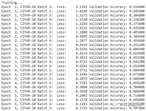
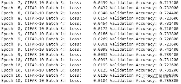
 1#Saving Model and Pathsave_model_path = './image_classification' 2print('Training...') 3with tf.Session() as sess: 4    # Initializing the variables 5    sess.run(tf.global_variables_initializer()) 6    # Training cycle 7    for epoch in range(epochs): 8        # Loop over all batches 9        n_batches = 510        for batch_i in range(1, n_batches + 1):11            for batch_features, batch_labels in load_preprocess_training_batch(batch_i, batch_size):12                train_neural_network(sess, optimizer, keep_probability, batch_features, batch_labels)13            print('Epoch {:>2}, CIFAR-10 Batch {}:  '.format(epoch + 1, batch_i), end='')14            print_stats(sess, batch_features, batch_labels, cost, accuracy)#Saving Model and Pathsave_model_path = './image_classification'
 2print('Training...')
 3with tf.Session() as sess:
 4    # Initializing the variables
 5    sess.run(tf.global_variables_initializer())
 6    # Training cycle
 7    for epoch in range(epochs):
 8        # Loop over all batches
 9        n_batches = 5
10        for batch_i in range(1, n_batches + 1):
11            for batch_features, batch_labels in load_preprocess_training_batch(batch_i, batch_size):
12                train_neural_network(sess, optimizer, keep_probability, batch_features, batch_labels)
13            print('Epoch {:>2}, CIFAR-10 Batch {}:  '.format(epoch + 1, batch_i), end='')
14            print_stats(sess, batch_features, batch_labels, cost, accuracy)
1# Save Model2    saver = tf.train.Saver()3    save_path = saver.save(sess, save_model_path)# Save Model
2    saver = tf.train.Saver()
3    save_path = saver.save(sess, save_model_path)
现在,TensorFlow图像分类的重要部分已经完成了,接着该测试模型。
测试模型
1import pickle 2import numpy as np 3import matplotlib.pyplot as plt 4from sklearn.preprocessing import LabelBinarizer 5def batch_features_labels(features, labels, batch_size): 6 """ 7 Split features and labels into batches 8 """ 9 for start in range(0, len(features), batch_size):10 end = min(start + batch_size, len(features))11 yield features[start:end], labels[start:end]12def display_image_predictions(features, labels, predictions, top_n_predictions):13 n_classes = 1014 label_names = load_label_names()15 label_binarizer = LabelBinarizer()16 label_binarizer.fit(range(n_classes))17 label_ids = label_binarizer.inverse_transform(np.array(labels))18 fig, axies = plt.subplots(nrows=top_n_predictions, ncols=2, figsize=(20, 10))19 fig.tight_layout()20 fig.suptitle('Softmax Predictions', fontsize=20, y=1.1)21 n_predictions = 322 margin = 0.0523 ind = np.arange(n_predictions)24 width = (1. - 2. * margin) / n_predictions25 for image_i, (feature, label_id, pred_indicies, pred_values) in enumerate(zip(features, label_ids, predictions.indices, predictions.values)):26 if (image_i < top_n_predictions):27 pred_names = [label_names[pred_i] for pred_i in pred_indicies]28 correct_name = label_names[label_id]29 axies[image_i][0].imshow((feature*255).astype(np.int32, copy=False))30 axies[image_i][0].set_title(correct_name)31 axies[image_i][0].set_axis_off()32 axies[image_i][1].barh(ind + margin, pred_values[:3], width)33 axies[image_i][1].set_yticks(ind + margin)34 axies[image_i][1].set_yticklabels(pred_names[::-1])35 axies[image_i][1].set_xticks([0, 0.5, 1.0])import pickle
2import numpy as np
3import matplotlib.pyplot as plt
4from sklearn.preprocessing import LabelBinarizer
5def batch_features_labels(features, labels, batch_size):
6 """
7 Split features and labels into batches
8 """
9 for start in range(0, len(features), batch_size):
10 end = min(start + batch_size, len(features))
11 yield features[start:end], labels[start:end]
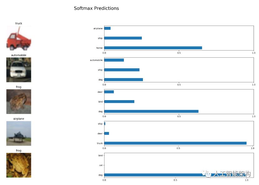
12def display_image_predictions(features, labels, predictions, top_n_predictions):
13 n_classes = 10
14 label_names = load_label_names()
15 label_binarizer = LabelBinarizer()
16 label_binarizer.fit(range(n_classes))
17 label_ids = label_binarizer.inverse_transform(np.array(labels))
18 fig, axies = plt.subplots(nrows=top_n_predictions, ncols=2, figsize=(20, 10))
19 fig.tight_layout()
20 fig.suptitle('Softmax Predictions', fontsize=20, y=1.1)
21 n_predictions = 3
22 margin = 0.05
23 ind = np.arange(n_predictions)
24 width = (1. - 2. * margin) / n_predictions
25 for image_i, (feature, label_id, pred_indicies, pred_values) in enumerate(zip(features, label_ids, predictions.indices, predictions.values)):
26 if (image_i < top_n_predictions):
27 pred_names = [label_names[pred_i] for pred_i in pred_indicies]
28 correct_name = label_names[label_id]
29 axies[image_i][0].imshow((feature*255).astype(np.int32, copy=False))
30 axies[image_i][0].set_title(correct_name)
31 axies[image_i][0].set_axis_off()
32 axies[image_i][1].barh(ind + margin, pred_values[:3], width)
33 axies[image_i][1].set_yticks(ind + margin)
34 axies[image_i][1].set_yticklabels(pred_names[::-1])
35 axies[image_i][1].set_xticks([0, 0.5, 1.0])
 1%matplotlib inline 2%config InlineBackend.figure_format = 'retina' 3import tensorflow as tf 4import pickle 5import random 6save_model_path = './image_classification' 7batch_size = 64 8n_samples = 10 9top_n_predictions = 510def test_model():11    test_features, test_labels = pickle.load(open('preprocess_training.p', mode='rb'))12    loaded_graph = tf.Graph()13    with tf.Session(graph=loaded_graph) as sess:14        # Load model15        loader = tf.train.import_meta_graph(save_model_path + '.meta')16        loader.restore(sess, save_model_path)
 2%config InlineBackend.figure_format = 'retina'
 3import tensorflow as tf
 4import pickle
 5import random
 6save_model_path = './image_classification'
 7batch_size = 64
 8n_samples = 10
 9top_n_predictions = 5
10def test_model():
11    test_features, test_labels = pickle.load(open('preprocess_training.p', mode='rb'))
12    loaded_graph = tf.Graph()
13    with tf.Session(graph=loaded_graph) as sess:
14        # Load model
15        loader = tf.train.import_meta_graph(save_model_path + '.meta')
16        loader.restore(sess, save_model_path)
1# Get Tensors from loaded model2        loaded_x = loaded_graph.get_tensor_by_name('input_x:0')3        loaded_y = loaded_graph.get_tensor_by_name('output_y:0')4        loaded_keep_prob = loaded_graph.get_tensor_by_name('keep_prob:0')5        loaded_logits = loaded_graph.get_tensor_by_name('logits:0')6        loaded_acc = loaded_graph.get_tensor_by_name('accuracy:0')# Get Tensors from loaded model
2        loaded_x = loaded_graph.get_tensor_by_name('input_x:0')
3        loaded_y = loaded_graph.get_tensor_by_name('output_y:0')
4        loaded_keep_prob = loaded_graph.get_tensor_by_name('keep_prob:0')
5        loaded_logits = loaded_graph.get_tensor_by_name('logits:0')
6        loaded_acc = loaded_graph.get_tensor_by_name('accuracy:0')
1# Get accuracy in batches for memory limitations2        test_batch_acc_total = 03        test_batch_count = 04        for train_feature_batch, train_label_batch in batch_features_labels(test_features, test_labels, batch_size):5            test_batch_acc_total += sess.run(6                loaded_acc,7                feed_dict={loaded_x: train_feature_batch, loaded_y: train_label_batch, loaded_keep_prob: 1.0})8            test_batch_count += 19        print('Testing Accuracy: {}'.format(test_batch_acc_total/test_batch_count))# Get accuracy in batches for memory limitations
2        test_batch_acc_total = 0
3        test_batch_count = 0
4        for train_feature_batch, train_label_batch in batch_features_labels(test_features, test_labels, batch_size):
5            test_batch_acc_total += sess.run(
6                loaded_acc,
7                feed_dict={loaded_x: train_feature_batch, loaded_y: train_label_batch, loaded_keep_prob: 1.0})
8            test_batch_count += 1
9        print('Testing Accuracy: {}
'.format(test_batch_acc_total/test_batch_count))
1# Print Random Samples2        random_test_features, random_test_labels = tuple(zip(*random.sample(list(zip(test_features, test_labels)), n_samples)))3        random_test_predictions = sess.run(4            tf.nn.top_k(tf.nn.softmax(loaded_logits), top_n_predictions),5            feed_dict={loaded_x: random_test_features, loaded_y: random_test_labels, loaded_keep_prob: 1.0})6        display_image_predictions(random_test_features, random_test_labels, random_test_predictions, top_n_predictions)7test_model()# Print Random Samples
2        random_test_features, random_test_labels = tuple(zip(*random.sample(list(zip(test_features, test_labels)), n_samples)))
3        random_test_predictions = sess.run(
4            tf.nn.top_k(tf.nn.softmax(loaded_logits), top_n_predictions),
5            feed_dict={loaded_x: random_test_features, loaded_y: random_test_labels, loaded_keep_prob: 1.0})
6        display_image_predictions(random_test_features, random_test_labels, random_test_predictions, top_n_predictions)
7test_model()
输出测试精度:0.5882762738853503
结语
如果你训练神经网络以获得更多功能,可能会具有更高准确度的结果。通过这个详细的实例,你应该已经可以使用它来分类任何类型的图像了。
长按订阅更多精彩▼

智能推荐
java 的 io流 读取文件里面 的内容(不定时更新)_java io读取文件内容-程序员宅基地
文章浏览阅读4.8k次,点赞4次,收藏29次。io流_java io读取文件内容
图像处理——过程全解析,配图超详细!-程序员宅基地
文章浏览阅读1.4k次。点击上方“小白学视觉”,选择加"星标"或“置顶”重磅干货,第一时间送达摘自先进测控之家《长着眼睛的机械手》课题摘要——利用图像处理技术,在50*50CM的区域内识别出5枚硬币(硬币位置任意),并且控制机械手逐一拾取5枚硬币,然后把5枚硬币逐一叠放到指定位置(指定位置随机)。图像处理过程详解——LabVIEWVision Assistant硬币位置识别算法分析与设计硬币的识别是本系统软件设计最为关..._图像处理
[ MATLAB ] 傅里叶变换(三):傅里叶变换_傅里叶变换可视化,plot3函数,matlab-程序员宅基地
文章浏览阅读774次,点赞35次,收藏25次。专题的前两篇文章([ MATLAB ] 傅里叶变换(二):傅里叶级数(复指数表示)),我们讨论了连续周期信号傅里叶级数的两种表示形式,初步建立了频谱的概念。然而,就实际经验而言,非周期信号才是主流。因此,这篇文章将讨论非周期连续信号的谱密度(通常简称为频谱),即大名鼎鼎的傅里叶变换FT,并用Matlab仿真加强理解。可以采用物理中的密度的方式类比谱密度的概念,从而理解傅里叶变换中谱密度的意义。不需要再执着于分量幅值的绝对大小,而是聚焦于相对大小。_傅里叶变换可视化,plot3函数,matlab
5G手机回归,鸿蒙份额激增,将进一步夯实三大操作系统的地位-程序员宅基地
文章浏览阅读360次,点赞8次,收藏8次。市调机构给出的数据指11月份华为手机在国内手机市场的份额达到14%,远超此前鸿蒙系统在国内手机操作系统8%的市场份额,这意味着随着华为5G手机的回归,鸿蒙系统的市占率将快速上涨。此前鸿蒙系统主要依靠华为手机的存量用户支持,在华为的推动下,诸多华为存量手机用户都转为了鸿蒙系统,这成为鸿蒙系统的第一批种子。随后华为在自己的穿戴设备、汽车等诸多产品上发展鸿蒙系统,还通过与美的等国内家电企业合作推广鸿蒙系...
openstack pike单机一键安装shell的方法(后期会转为python)-程序员宅基地
文章浏览阅读183次,点赞9次,收藏2次。#VM虚拟机8G内存,安装完毕,半个小时左右#在线安装#环境 centos 7.4.1708 x86_64#在线安装openstack pikePS: 排版问题,还在研究。wangleideMacBook-Pro:Downloads wanglei$ cat pike.install.sh#!/bin/sh# openstack pike 单机 一键安装# 环..._ali-pike.repo
通过formData数据发送ajax请求-程序员宅基地
文章浏览阅读1.9k次。formData1.创建一个formData对象var fd = new FormData(‘form表单’);(创建formdtata对象的小括号里面,就是需要一个form表单dom对象)。2.往fd对象中添加对象fd.append(‘sex’,‘男’);3.formData里面就会有form表单中 有name属性的这些标签的取值。//键值对形式console.log(fd.ge...
随便推点
ceph中的radosgw相关总结_radosgw -c-程序员宅基地
文章浏览阅读627次。https://blog.csdn.net/zrs19800702/article/details/53101213http://blog.csdn.net/lzw06061139/article/details/51445311https://my.oschina.net/linuxhunter/blog/654080rgw 概述Ceph 通过radosgw提供RES..._radosgw -c
前端数据可视化ECharts使用指南——制作时间序列数据的可视化曲线_echarts 时间序列-程序员宅基地
文章浏览阅读3.7k次,点赞6次,收藏9次。我为什么选择ECharts ? 本周学校课程设计,原本随机佛系选了一个51单片机来做音乐播放器,结果在粗略玩了CN-DBpedia两天后才回过神,课设还没有开始整。于是懒癌发作,碍于身上还有比赛的作品没交,本菜鸡对硬件也没啥天赋,所以就直接把题目切换成软件方面的题目。写python的同学选择了一个时间序列数据的可视化曲线程序设计题目,果真python在数据可视化这一点性能很优秀。..._echarts 时间序列
ApplicationEventPublisherAware事件发布-程序员宅基地
文章浏览阅读1.6k次。事件类:/** * * * @className: EarlyWarnPublishEvent * * @description:数据风险预警发布事件 * * @param: * * @return: * * @throws: * * @author: lizz * * @date: 2020/05/06 15:31 * */public cl..._applicationeventpublisheraware
自定义View实现仿朋友圈的图片查看器,缩放、双击、移动、回弹、下滑退出及动画等_imageview图片边界回弹-程序员宅基地
文章浏览阅读1.2k次。如需转载请注明出处!点击小图片转到图片查看的页面在Android开发中很常用到,抱着学习和分享的心态,在这里写下自己自定义的一个ImageView,可以实现类似微信朋友圈中查看图片的功能和效果。主要功能需求:1.缩放限制:自由缩放,有最大和最小的缩放限制 2居中显示:.若图片没充满整个ImageView,则缩放过程将图片居中 3.双击缩放:根据当前缩放的状态,双击放大两倍或缩小到原来 4.单指_imageview图片边界回弹
PreScan第二课:构建实验_prescan坐标系-程序员宅基地
文章浏览阅读5.5k次,点赞8次,收藏37次。为了自己和他人学习的需要,建了一个PreScan的QQ群:613469333(已满)/ 778225322(可加),加群前请私聊群主(QQ:2059799865)加入。群管理需要花费时间和精力,为了鼓励管理员和群成员积极互动,入群需交¥9.99的群费。目录1 Conventions坐标系统2 Roads3 Path&trajectories路径和轨迹3.1 Pat..._prescan坐标系
三分钟带你掌握 CSS3 的新属性_采用css转换,边框阴影等新特性完成css3偏光图像画廊设计-程序员宅基地
文章浏览阅读3.8w次,点赞9次,收藏10次。1. css3简介CSS 用于控制网页的样式和布局,CSS3 是最新的CSS标准,CSS3 完全向后兼容,因此您不必改变现有的设计。浏览器通常支持 CSS2,但是现在大部分浏览器也实现了css3的很多特性。CSS3 被划分为模块。其中最重要的 CSS3 模块包括:选择器框模型背景和边框文本效果2D/3D 转换动画多列布局用户界面2. css3边框2.1 边框圆角Internet Explorer 9+ 支持 border-radius 和 box-shadow 属性。Fir_采用css转换,边框阴影等新特性完成css3偏光图像画廊设计